This HTML edition contains selectable text extracted from the original PDF. Layout-aware OCR was used to recover reading order, figures and equations; minor recognition errors may remain. Consult the PDF for the authoritative layout, figures and equations.
SOME RESULTS OF APPLYING SCALE-UP EQUATIONS TO PREDICT
SLURRY PRESSURE DROP IN LARGE PIPES.
A.D. Thomas.
M.D. Research Company Pty. Limited, North Ryde,
N.S.W., Australia.
Summary
Scale-up of slurry pressure drop to large diameter pipes is discussed with interest concentrating on slurries having particles with free settling velocities of from .01 to .15 m/s. Several slurries are tested for scale-up by using the results obtained in 50 mm and 100 mm pipes to predict the behaviour in 300 mm nominal diameter pipes and comparing this prediction with experimental data from external sources. The scale-up procedure recently proposed by the author is shown to be superior to more commonly used methods.
To date this scale-up procedure has mainly been tested on slurries having particles of narrow size distribution. Problems encountered when extending the method to wide size distributions are discussed and illustrated by an example.
Finally it is shown how available evidence suggests that this scale-up procedure can be used as the basis for a new empirical approach to pressure drop prediction without pipe loop testing.
Available methods of predicting slurry pressure drop, especially in large pipes, are still far from satisfactory and pipe loop tests usually need to be performed to confirm the prediction. If these pipe loop tests are performed in pipes of smaller diameter than the planned pipeline the results must be scaled up to the larger diameter. The literature on scale-up methods is very sparse with the main contribution being by Bowen (Ref.1.). The Bowen scale-up procedure is suitable for homogeneous type slurries which fortunately are the ones of most interest as far as long distance pipelines are concerned. However there are numerous situations where it is desirable to pump slurries having coarser particles such that the slurry is of a settling nature. Apart from a recent paper by the author (Thomas, Ref.2) there does not appear to have been any papers published concerned specifically with scale-up procedures for such slurries. For very coarse slurries the Durand equation (Ref.3) would be applicable and could be used for scale-up but such slurries are generally not of great interest. Of most interest are slurries which can be termed "moderately settling". These slurries will tend towards homogeneous type behaviour at high velocities but will exhibit "settling" tendancies at lower velocities where they will flow in a heterogeneous manner. Such slurries will be described here as semi-heterogeneous. Slurries with particles having free settling terminal velocities, , of from 0.01 to 0.15 m/s will behave in such a manner. For sand particles this would mean sizes from 0.1 mm to 1 mm.
2. AVAILABLE SCALE-UP EQUATIONS FOR SEMI-HETEROGENEOUS SLURRIES.
For very fine particles travelling as a homogeneous suspension with possible non-Newtonian behaviour the Bowen scale-up equation can be used:
Where is the pressure gradient
, and are constants for a particular slurry at a particular concentration and are determined from the pipe loop tests.
is pipe diameter
is mean velocity of mixture
Kenchington (Refs. 4 and 5) has discussed the use of this method and the problems likely to be encountered in its application.
For slightly larger particles where surface chemistry effects are negligible and at relatively low concentrations Newtonian behaviour will be observed and equation (1) will reduce to:
For smooth pipe flow from the Blasius equation.
For rougher pipes is a reasonable figure.
Since the water pressure drop, , can be described by an equation similar to equation (3) the scale-up equation can be written as:
Equation (4) would be applicable for particles having m/s. For sand S.G. = 2.65 this represents particles less than about 100 microns. This equation could therefore be used as a scale-up equation in the fine particle region of the semi-heterogeneous slurry range. For increasingly coarser particles it will progressively underestimate the pressure gradient but will provide a lower limit. At high flow velocities where the slurry behaves more homogeneously equation (4) would be expected to provide an increasingly more accurate scale-up method.
At the coarse particle end of the semi-heterogeneous slurry range, where approaches 0.15 m/s, the Durand equation could be expected to provide a reasonable scale-up equation. The Durand equation can be expressed as
For a particular slurry at a particular concentration this reduces to:
Approximating by equation (3) this becomes
where , and are constants.
Equation (7) should therefore be suitable for scaling-up semi-heterogeneous slurries at the coarse particle end of the range. For sand particles this will be for sizes approaching 1 mm. For particles finer than this it should provide an upper limit.
Thomas (Ref.2) has proposed a scale-up equation for the entire semi-heterogeneous regime.
In this equation , and are constants which need to be determined from pipe loop tests.
Because the exponent of in the first term is not fixed tests are necessary on the same slurry in at least two different pipe sizes. This is in contrast to equations (4) and (7) where the scale-up equation can be obtained from the results of tests in only one diameter pipe.
Charles (Ref.6) proposed an equation which allows for a gradual transition from heterogeneous to homogeneous behaviour with increasing velocity. For scale-up purposes his equation would be similar to equation (8) except that the value of would be fixed at +.3. This places the same limitation on his equation as is imposed on the Durand equation.
3. EXAMPLES OF SCALE-UP.
Equations (4), (7) and (8) will now be applied to three different slurries of the semi-heterogeneous type. The results of tests in small diameter pipes will be used to obtain the constants in these equations which will then be used to predict the pressure drop in a large diameter pipe. The three predictions will be compared with the measured pressure drop to assess the relative merits of the three methods.
Slurry A
Sand S.G. = 2.65
by volume
mm
m/s
The size distribution of this sand slurry is shown in Figure 1. Reference 7 presents the results of tests of this slurry in pipe sizes from 52 mm to 315 mm. The results for the 52 mm and 107 mm pipes are shown in Fig. 2. At the higher velocities in the smaller pipe the curve is tending towards a straight line indicating the approach of homogeneous behaviour. Fig. 3 shows the same results plotted as versus velocity. The data do not follow a straight line, either of slope + 1.8 as suggested by equation 4 or of slope - 1.2 as suggested by equation 7 but follow the characteristic curved path of a semi-heterogeneous slurry best described by equation 8. Non-linear least squares estimation of the parameters , and of equation 8 using this data resulted in the scale-up equation:
where
&
are in mm water /m
is in mm
and
is m/s
This equation resulted in the curves as shown fitted to the data of the 52 mm and 107 mm pipes in Fig.3. Using this equation the behaviour in a 315 mm diameter pipe can be predicted and is also shown in Fig.3. Also shown as dashed lines are the predictions obtained by scaling-up using equations 4 and 7. In applying these two equations the slurry was assumed to behave most homogeneously at the highest velocity in the 52 mm pipe. This data point then supplied the constant in equation 4. The lower velocity points in the 107 mm pipe were used to obtain the constant in equation 7. Experimental data obtained in the 315 mm pipe lie between that predicted by equations 4 and 8. Equation 4 predicts values of - between 25% and 50% below the measured value, while equation 7 overpredicts by more than 100%. Equation 8 overpredicts by 30% (about 12% in ).
Slurry B
Data was available from tests on an iron sand ( to ) slurry in a 311 mm pipe. (Ref.8). This iron sand was from the Taharoa deposits in the North Island of New Zealand. To simulate this slurry for purposes of scale-up tests were conducted on an ilmenite beach sand slurry of similar particle size in the author's 53 mm and 105 mm diameter pipe loops. The size distribution of the ilmenite is shown in Fig.1 and is seen to lie between the two size distributions supplied by New Zealand Steel Limited shown dashed. The results of the pipe loop tests for are shown in Fig. 4 plotted as - versus velocity. Once again semi-heterogeneous type behaviour is evident but this slurry is noticeably more heterogeneous in behaviour than the previous sand slurry.
Equations 4 and 7 applied to this data in the same manner as previously resulted in the dashed lines as predictions for the behaviour in a 311 mm pipe. The constants in equation 8 were determined to be , , which resulted in the predicted curve as shown. Equation 4 is seen to give a prediction of between 40% and 50% of the measured values while equation 7 overpredicts by between 5% and 40%. Equation 8 predicts values within 4% and 10% of the measured values.(2% to 4% in ).
Slurry C
Fuhrboter (Ref.9) has presented the results of tests in a 300 mm pipe on a sand slurry of median particle size 0.84 mm. The size distribution is shown in Fig.1 as a dashed line. To simulate this slurry tests were performed by the author using -16 + 30 mesh sand. This sand was of smaller median particle size but because the slurry was pumped at a high temperature ( ) the values were expected to be approximately the same. Tests were run at a concentration of 16.5% by volume in the 53 mm and 105 mm test loops. This slurry was more heterogeneous in behaviour than the previous two as evidenced by the - versus plots of Fig.5 which much more nearly follow a straight line of slope -1.2. Scatter is large and might be expected with such coarse particles. The constants in equation 8 were found to be , , , resulting in a predicted curve not too different from that predicted using equation 7. Both of them overpredict by some 35%. (20% overprediction of ) while equation 4 underpredicts by about the
same amount. However the tests in the two smaller pipes were for whereas the data for the large pipe is for . Allowance for this would reduce the error in the predictions of using equations 7 and 8 to about 20% - 25%.
Discussion on above scale-up examples.
These three examples illustrate the advantages of equation 8 as a scale-up equation. In all cases equation 8 provides a closer prediction of the pressure gradient in a large pipe than either equation 4 or 7. Of more importance than the percentage errors involved however is the way in which the experimental data in the large pipes follows much more closely the curve predicted by equation 8 than the straight line relationships predicted using equations 4 and 7.
4. SCALE-UP OF SLURRIES HAVING WIDE PARTICLE SIZE DISTRIBUTIONS.
The above three examples all have narrow particle size distributions. In Ref. 2 it was shown how the scale-up procedure using equation 8 worked equally well for a sand slurry having a wide particle size distribution. Data taken from Ref. 7 was used in that case and the results for 107 mm and 158 mm pipes were used to scale-up to a 263 mm pipe.
An attempt was made to simulate this slurry in the author's 53 mm and 105 mm pipe loops so that the scale-up method could be tested for this wide size distribution slurry over a greater range of pipe diameters. The size distributions of three such tests are shown in Figure 6. These are for one test in the 53 mm pipe and two separate tests in the 105 mm pipe all at the same concentration of 25% by volume. The full line taken from Ref. 7 shows the size distribution of the slurry tested in the 263 mm pipe. Obviously the simulation of this size distribution was not as good as would have been hoped although the coarse portion of the distribution is reasonably well simulated. Nevertheless the results were plotted as versus and are shown in Fig. 7. It is obvious that the two slurries tested in the 105 mm pipe (sands 1 and 2) produce significantly different results even though their size distributions at first glance do not seem markedly different. The coarser particle slurry (sand 1) produced some 25% above the finer particle slurry (sand 2). A similar difference would be expected for mm as is predicted by applying equation 7 to the two results. (dashed lines in Fig. 8) However when equation 8 is applied the results from two pipe sizes must be used and if the size distributions in the two pipes are at all different the error in the prediction will be magnified. This is illustrated in Fig. 8 where the full lines show the results of fitting equation 8 firstly to the data for sands 1 and 3 and then for sands 2 and 3. The resulting values of the constants were respectively:
The large difference in the value of the exponent has resulted in the first combination predicting values some 60% above that predicted by the second combination. This serves to highlight the necessity for the size distributions in the two pipes to be as close as possible if scale-up using equation 8 is to be accurate. With wide size distributions this may not be easy to attain as the variation in flow rate with pipe size may cause different size distributions to be delivered even though the input mixtures are the same in both cases.
Noting the differences in behaviour of sands 1 and 2 in Fig. 7 caused by a relatively small difference in size distribution it is obvious that the sand tested in the 263 mm pipe (full line on Fig. 6) would give considerably lower pressure drops than any of the three sands 1, 2 and 3. This is indeed suggested by Fig. 8.
It is apparent that the success of the scale-up procedure using equation 8 will depend on how closely the particle size distribution is controlled. For narrow size distributions this is no problem but it becomes increasingly more difficult as the size distribution is widened.
In the scale-up equation 8 it is reasonable to assume that both and are functions of , , and , being the of the solids. Figure 9 shows the exponent plotted against for the narrow size distribution slurries tested to date. The data for the sand slurries having m/s were obtained from Ref. 7. The data points for and 24% for this sand represent the resulting from the fitting of equation 8 to data from 52 mm, 107, 158, 208, 263 and 315 mm pipes. The data point for represents data from 52, 107 and 263 mm pipes. All other points were obtained using data from 50 and 100 mm pipes only. The m/s results used data from Ref. 10 while the other three points were obtained from tests performed by the author.
Figure 9 indicates that for a given value of and a unique value for can be obtained. From the ilmenite results it appears that the specific gravity of the solids is entirely accounted for by the value so that the curves of Figure 9 would seem to be valid for all specific gravities. The general trends evident from this figure are that at high values of approaches the Durand value of +.3 but as the is reduced becomes more negative. For the same value higher concentrations give a more negative value of , i.e. more homogeneous behaviour as would be expected.
Figure 10 shows a plot of versus . Once again the ilmenite results lie on the same curve as for the ordinary sand suggesting that the effect of specific gravity is entirely allowed for by plotting in this manner.
In both figures the data point for m/s ( ) would seem to be slightly out of place. The difficulties associated with testing a slurry of such coarse particles as illustrated by the scatter of data points of figure 5 could explain this discrepancy.
Figures 9 and 10 are obviously far from complete and can only be regarded as tentative at this stage. Further tests on a number of slurries having narrow particle size distributions are planned. Nevertheless in their present form Figs. 9 and 10 do permit a reasonable estimate of and in equation 8, for the range of variables tested. The second term in this equation, , would be expected to be largely independent of and could be approximated by . The complete equation will then enable pressure gradient prediction a priori from particle properties. Using Figs. 9 and 10 in their present form and be predicted generally within 30% for the range of variables tested. This can be compared with the results of applying the Durand equation (eqn. 5) with to slurry A in a 315 mm pipe. It overpredicts by more than 500%.
Extension to slurries having a wide particle distribution.
Extension of the above method to slurries having a wide size distribution would require an estimate of an equivalent value of , to use in Figs. 9 and 10. It is not immediately clear how could be selected. Until this is resolved Figs. 9 and 10 could be used as an aid to scale-up in the following manner.
- (a) Tests are performed on the slurry in one pipe.
- (b) From this data the value of in equation 8 can be determined although and cannot be individually determined.
- (c) Figs. 9 and 10 can be used to obtain a plot of versus for this particular pipe diameter. From this plot it is then possible to obtain an equivalent for the observed value of .
- (d) Using this and can be determined from Figs. 9 and 10 and the complete scale-up equation obtained.
The scale-up method proposed recently by the author (Thomas Ref. 2) equation 8, has been applied to a number of slurries covering the full range of semi-heterogeneous behavious and shown to give better predictions and to describe the experimental behaviour far more satisfactorily than either the Durand equation or the homogeneous model. Data available to date suggests that curves similar to Figs. 9 and 10 offer promise of providing a means of accurate prediction of slurry pressure drop from the particle properties of and without scale-up from pipeline testing being necessary. Even in their present tentative form these two figures allow more accurate prediction of pressure gradient than presently available alternative methods but only for slurries having narrow particle size distributions.
For slurries having wide particle size distributions the scale-up procedure using equation 8 would seem to be equally applicable. However extreme care is necessary to ensure that the size distributions in the two pipe sizes used are exactly the same since any differences will magnify the errors considerably. This may limit the use of this scale-up method for these slurries so an alternative procedure using Figs. 9 and 10 whereby an equivalent value of is found from tests in only one pipe has been suggested.
Acknowledgements.
The author gratefully acknowledges and thanks
- 1. M.D. Research Company Pty. Limited for permission to publish this paper.
- 2. New Zealand Steel Limited for supplying the data on the iron sand slurry.
References.
- 1. Bowen, R.L. (Jnr) Series of articles in Chem. Engng June 12, p 243, June 26, p 127, July 10, p 147, July 24, p 143, August 7, p 129, August 21, p 119, 1961.
- 2. Thomas, A.D. "Scale-up methods for pipeline transport of slurries". To be published in Int. J. of Mineral Processing.
- 3. Durand, R. "Basic relationships of the transportation of solids in pipes - experimental research". Proc. Minnesota Int. Hyd. Convention, pp89-103, Int. Assoc. for Hyd. Research, 1953.
- 4. Kenchington, J.M. "The design of large pipelines for cement slurries" 2nd Int. Conf. on the Hyd. Trans. of Solids in Pipes, Paper C4. Org. by Brit. Hydromech. Res. Assoc., Univ. of Warwick, England 20 - 22nd Sept., 1972.
- 5. Kenchington, J.M. "The prediction of pressure drop in slurry pipelines" Multiphase flow Symposium organized jointly by I. Ch. E. and I. Mech. E., Univ. of Strathclyde, Glasgow, 1974.
- 6. Charles, M.E. "Transport of solids by pipeline" 1st Int. Conf. on the Hyd. Trans. of Solids in Pipes, Paper A3. Org. by Brit. Hydromech. Res. Assoc., Univ. of Warwick, England 1st - 4th September, 1970.
- 7. Schriek, W., Smith L.G., Haas, D.B., and Husband, W.H.W. "Experimental studies on the transport of two different sands in water in 2, 4, 6, 8, 10 and 12 inch pipelines" Report VII of a series of reports on Experimental Studies on Solids Pipelining of Canadian Commodities for the Canadian Transport Commission and the Transportation Development Agency. Tests performed by Saskatchewan Research Council. 50pp 1973.
- 8. Private communication from New Zealand Steel Ltd. via Prof. A.J. Raudkivi, Univ. of Auckland, N.Z. 1975.
- 9. Fuhrboter, A. "Über die Forde ung von Sand-Wasser-Gemischen in Rohrleitungen" Mitteilungen des Franzis Instituts für Frund- und Wasserbau der Technischen Mechanik Hannover. No.19 152pp, 1961. (In German.)
10.
Shook, C.A., Schriek, W., Smith, L.G., Haas, D.B., and Husband, W.H.W.
"Experimental studies on the transport of sands in liquids of varying
properties in 2 and 4 inch pipelines" Report VI of a series of reports on
Experimental Studies on Solids Pipelining of Canadian Commodities for the
Canadian Transport Commission and the Transportation Development Agency.
Tests performed by Saskatchewan Research Council 158 pp, 1973.
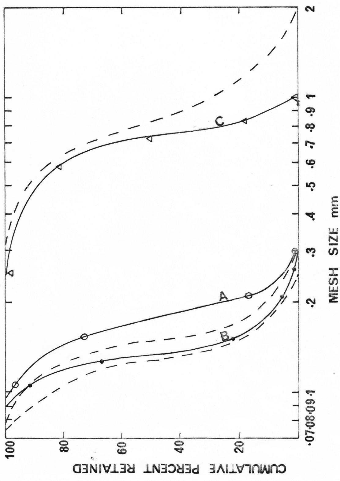
Fig.1. Size distribution of slurries A, B and C
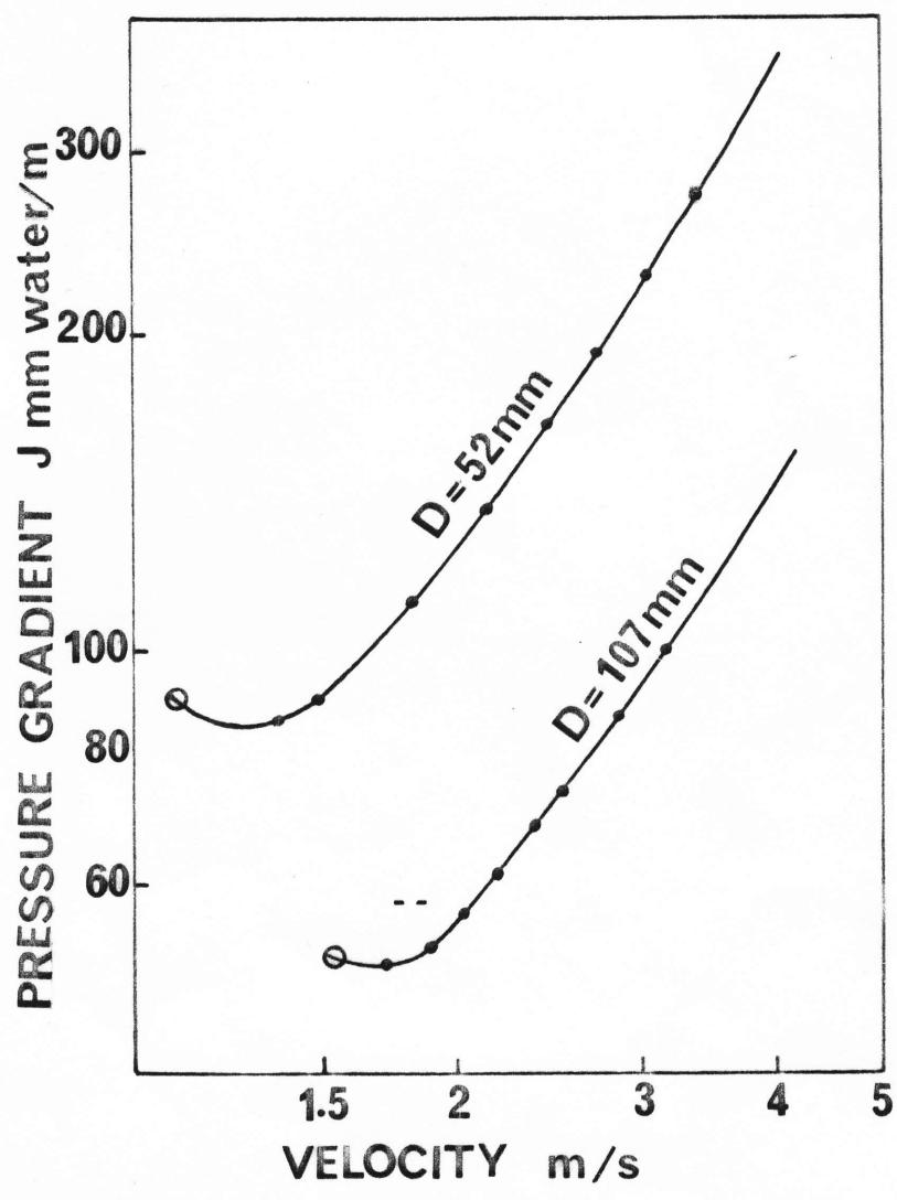
Fig. 2. Observed pressure gradient of slurry A
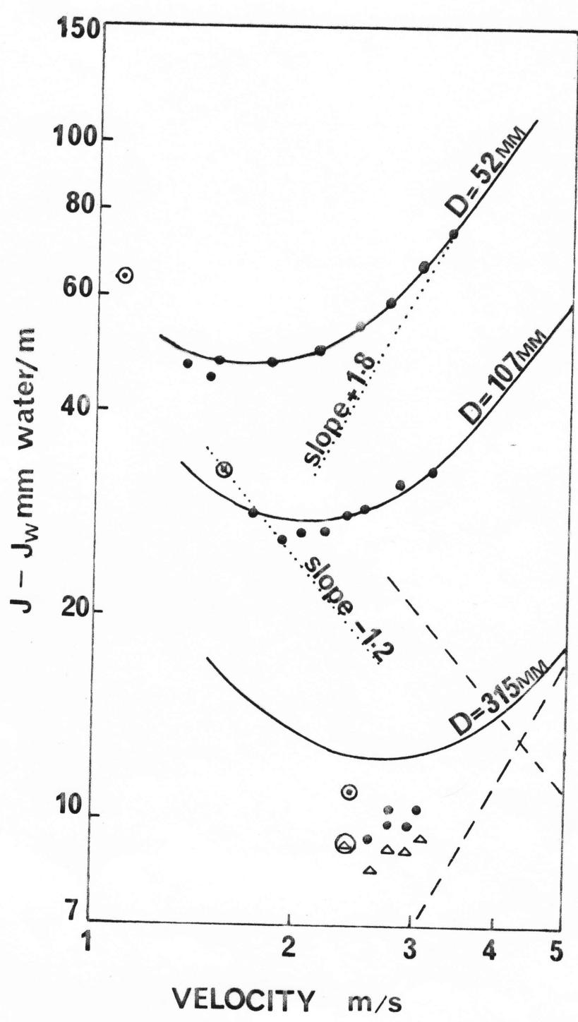
Fig 3. Scale-Up of slurry A. Ringed points indicate stationary bed deposit. For , , .
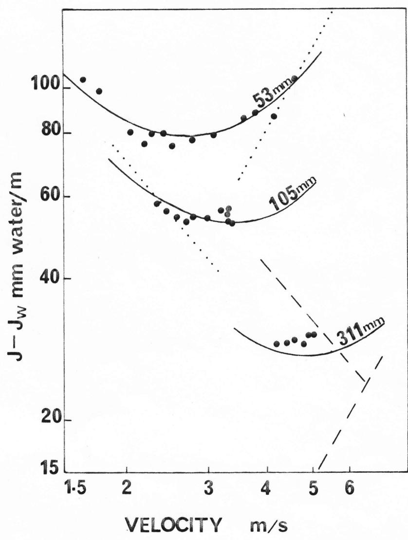
Fig 4. Scale-Up of slurry B
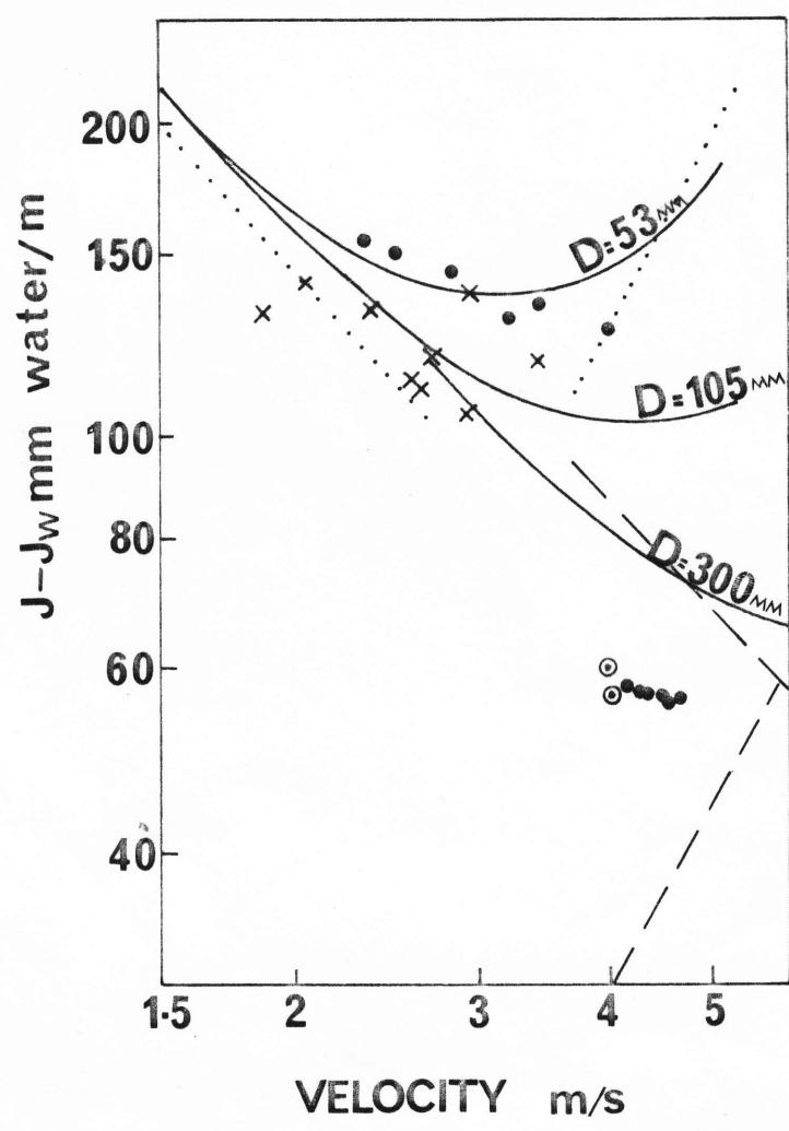
Fig 5. Scale - Up of slurry C
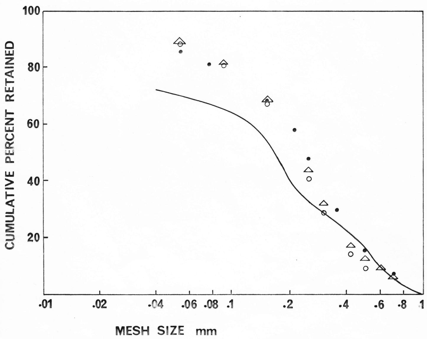
Fig 6. Size distribution of wide size distribution slurry.
• D=105mm (Sand 1), D=105mm (Sand 2), D=53mm (Sand 2)
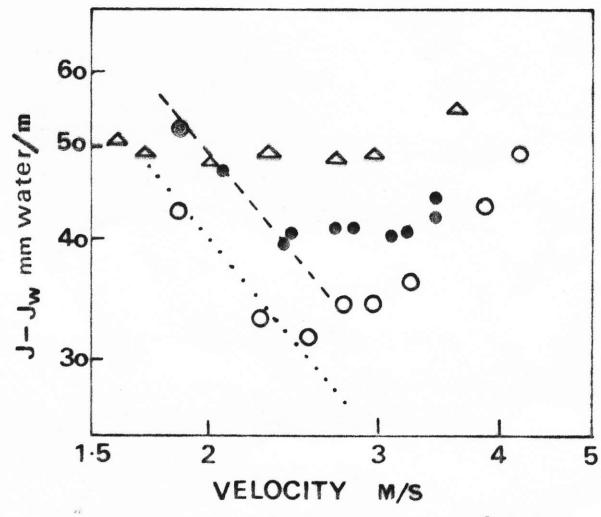
Fig 7 Behaviour of sand 1, 2 & 3
• Sand 1, ○ Sand 2, △ Sand 3
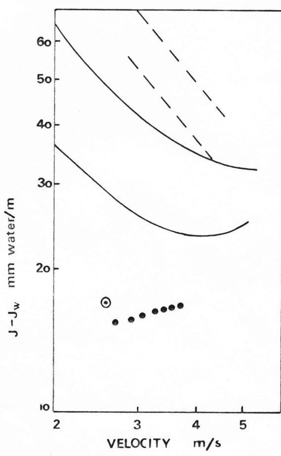
Fig 8. Results of scale - up to mm using two combinations of sand
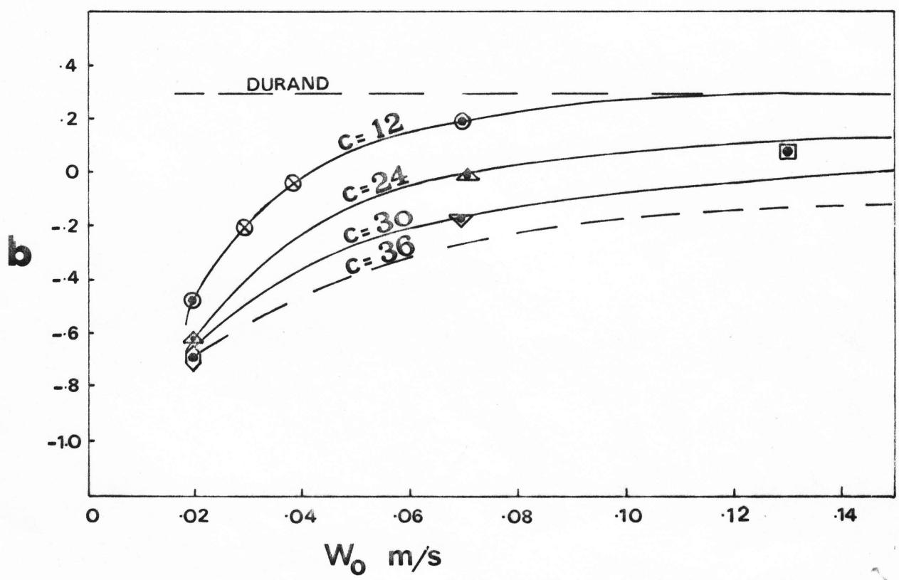
Fig 9. Variation of b (eqn 8) with
- • Sand SG=2.65 , Ilmenite SG=4.50 ,
- c=12 , c=16.5 , c=24 , c=30 , c=36.
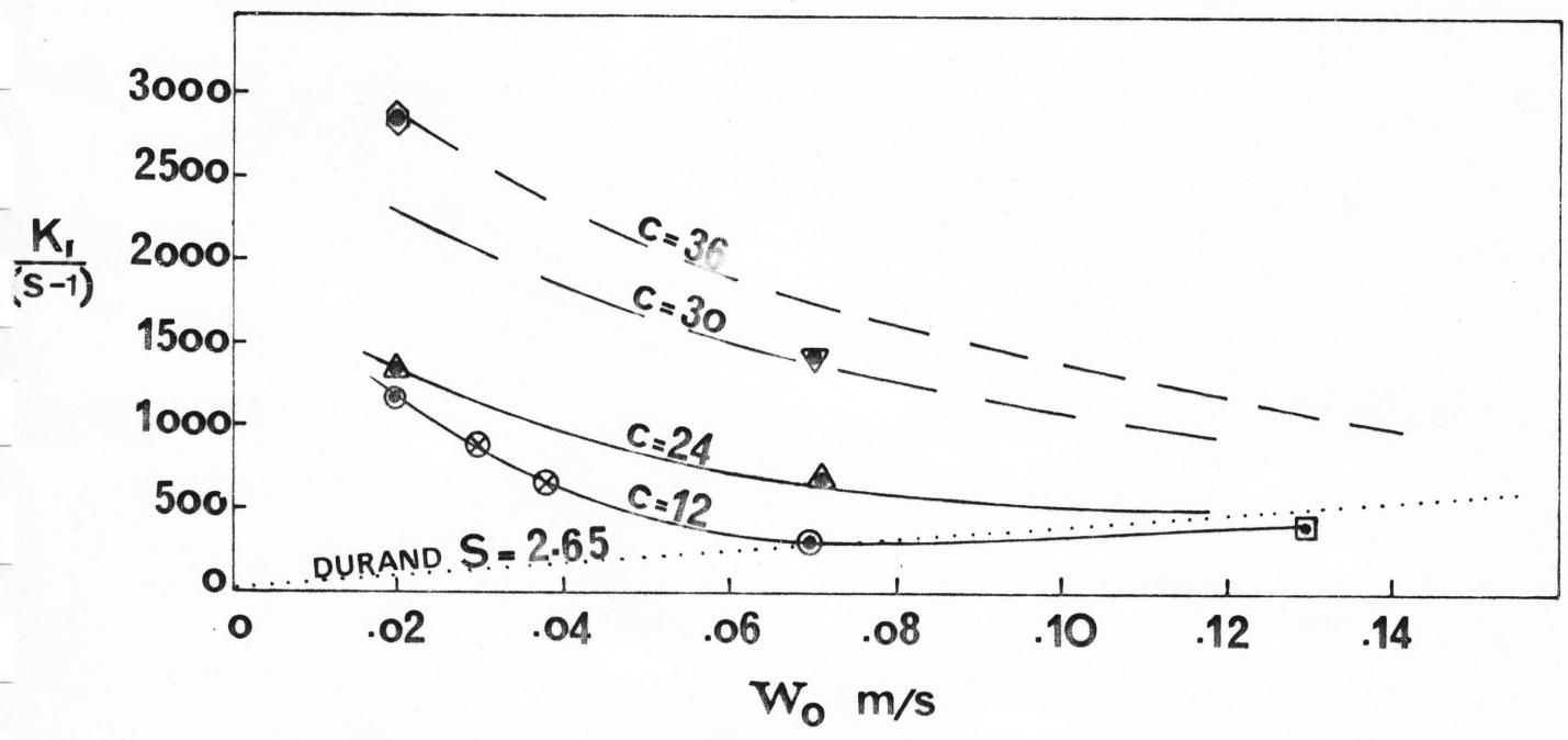
Fig 10. Variation of (eqn 8) with .
- • Sand S.G.=2.65, Ilmenite S.G.=4.50,
- , , , , .