Scale-up methods for pipeline transport of slurries

Page 1

International Journal of Mineral Processing, 3 (1976) 51—69 • Elsevier Scientific Publishing Company, Amsterdam - Printed in The Netherlands

SCALE-UP METHODS FOR PIPELINE TRANSPORT OF SLURRIES

A.D. THOMAS

M.D. Research Company Pty, Ltd., North Ryde, N.S. W. (Australia) (Received April 14, 1975; revision accepted July 25, 1975)

ABSTRACT

Thomas, A.D., 1976. Scale-up methods for pipeline transport of slurries. Int. J. Miner. Process., 3: 51-69. The behaviour of different types of slurries is discussed under two main headings: homogeneous and heterogeneous. Methods of scaling-up pressure-drop data obtained in small-diameter pipes to large-diameter pipes are discussed and recommendations are made as to the best method to use for different slurries. For slurries which flow in a homogeneous manner, the Bowen scale-up procedure is recommended. In the case of heterogeneous flowing slurries it is shown how their behaviour in small pipes can be used to further classify them into semi-heterogeneous or fully heterogeneous types. For scale-up of the latter, the Durand type of equation is recommended. For the semi-heterogeneous slurries, which are often the ones of most commercial interest, it is shown how no existing correlations adequately describe their behaviour. A new scale-up equation is proposed for these slurries. All scale-up methods are illustrated by using experimental data obtained in pipes from 50 mm to 300 mm diameter. It is shown how tests in pipes of diameter no greater than 100 mm can accurately predict pressure drop to within 15% in pipes up to three times this diameter.

INTRODUCTION

The transport of minerals by pumping them along pipelines in slurry form is used extensively in the minerals processing industry. The majority of these pipelines are of short distance mainly within a particular plant. However, increasing interest is being shown in long-distance pipelines as an alternative to conventional means of transport such as road and rail. As the length and capital cost of a pipeline increases, there becomes an increasing necessity for accurate prediction of the slurry pressure drop. At the present time there is no method available which will allow accurate prediction of the pressure drop from bench-scale test data of parameters such as viscosity, particle size, particle settling rates etc. Because of this, if the pressure drop in a large-diameter

pipe is to be predicted with any accuracy (say better than 50%) it is necessary

to perform pipe loop tests. Experimental pipe loops usually consist of pipes of three or four different diameters with the largest often being around

Page 2

52

150 mm. To apply the results of tests done in these pipes to larger diameter pipes it is necessary to use scale-up laws. In this paper the various methods currently available for scale-up are reviewed and discussed and recommendations are made as to the best method to use for different types of slurries. Experimental results obtained in commercial sized pipes are used to illustrate the methods.

CLASSIFICATION OF SLURRIES

Solid-liquid mixtures can be classified according to the manner in which they flow in a horizontal pipe. If, in the velocity range of commercial interest, a slurry flows with a uniform concentration of particles about the pipe axis it can be classified as a homogeneous slurry. Such a slurry will flow as a singlephase fluid with viscosity and density different from that of the carrier liquid. Into this category naturally fall the non-settling slurries, i.e., those slurries from which particles will not settle even if they are left standing for a long period of time. A slurry of this type would have most particles less than 10 or 20 u. For such slurries turbulence is not required to suspend the particles so that they can flow even in the laminar regime without settling of particles occurring. However, also included in the homogeneous category are some slurries with larger particles which do require turbulence to keep them suspended. Such slurries will flow in a homogeneous manner under turbulent conditions in the velocity range of commercial interest, say above 1 m/sec for pilot-scale pipes, but at velocities below this, settling of particles will occur. This settling could occur while the flow is still turbulent in which case it would be due to insufficient intensity of turbulence for maintenance of the larger particles in suspension or it could occur because of transition to laminar flow. The second class of slurries termed heterogeneous slurries, are those which, in the velocity range of commercial interest, will flow with a non-axisymmetric concentration distribution. Such slurries do not behave as a single-phase fluid and the flow is a true two-phase flow in that the solid and liquid phase retain their identity. It should be noted that if there is a wide particle size distribution the fine particles may be transported homogeneously whilst the coarser particles could be transported heterogeneously.

SCALE-UP PROCEDURES FOR THE FLOW OF HOMOGENEOUS SLURRIES

Homogeneous slurries sometimes behave as Newtonian fluids but more often they exhibit non-Newtonian properties such as a yield stress and a noninear stress-shear rate relationship, especially at high concentrations. The problem of pressure-drop prediction of a homogeneous slurry is therefore on of pressure-drop prediction for a non-Newtonian fluid. If, from viscometer tests, a rheological model of this slurry is obtained there are a number of

Page 3

53

methods available which will allow prediction of the laminar and turbulent pressure drops and the transition velocity between the two regimes. The bestknown of these methods is that due to Dodge and Metzner (1959) which applies to a powerlaw fluid without a yield stress. Cheng (1970) has modified their method to accommodate a more general fluid with a yield stress and has applied it to a large number of commercial pipelines. More recent theories are due to Hanks and Dadia (1971) and Kemblowski and Kolodziejski (1973). Kenchington (1974) has compared the predictions of all the above methods with experimental pressure drops for clay and kiln feed slurries for pipe diameters ranging from 16 mm to 329 mm. He found that all these methods predicted the turbulent pressure drop with reasonable accuracy (30%). However prediction of the laminar pressure drop and the transition velocity was not so accurate. Whilst there are very few commercial slurry pipelines operating in the laminar regime, a lot of those flowing in the turbulent regime do operate close to the transition region. Any error in prediction of the transition velocity will cause large errors in pressure-drop prediction for these slurries. Kenchington attributed this inaccuracy in the transition velocity to wall slip effects which cannot be allowed for from viscometer tests. This "slip" effect is caused by the formation of a particle-free layer near the wall giving reduced values of the local shear stress. It should also be noted that the viscometer tests as performed by Kenchington were done with sophisticated equipment and great care. Obtaining accurate and meaningful results from viscometer tests on slurries is not easy and although the bench-scale equipment used is small and requires only a small slurry sample the number of man hours used can be high. Because of these reasons pipe-loop tests are invariably also required if high accuracy is desired. Bowen (1961) has presented a complete design procedure for scaling-up small pipe results on a slurry at a particular concentration to large pipes in both the laminar and turbulent regimes. In the laminar regime he uses the method of Metzner and Reed (1955). This method is applicable to any purely viscous liquid, i.e., a log-log plot of wall shear stress Tw against 8 V/D will correlate the data for different pipes providing there is no slip effect. For a power-law fluid this plot will be straight line. If slip occurs plots of data from different pipes will be displaced and this effect will need to be allowed for in any scale up procedure. This is discussed by Kenchington (1974) and Harris and Quader (1971). For turbulent pressure drop prediction Bowen's method uses small-scale turbulent data for scaling-up. It has as its basis the assumption that for a non- Newtonian fluid, the Blasius equation for the turbulent friction factor can be generalised. The Blasius friction factor for a Newtonian fluid is valid for the range of Reynolds Numbers of interest in slurry flow. This is given as: f = 0.079 (D Vp / 4) - * (1)

Page 4

54

Combining this with the Fanning equation: J= 2fp V2/D (2) one obtains: J=2 A V2-× D-1-X p1-* u* (3) where J is the pressure gradient; V is mean slurry velocity; D is the pipe diameter, and A is a constant; x = 0.25 for flow in smooth pipes. For a particular Newtonian fluid p and u are constant and eq. 3 becomes: J= A, V2-× D-1-x (4) For flow in rough pipes x = 0.20

-

The Hazen and Williams formula gives x = 0.15. The actual value of x can be determined from pipe-loop tests but in any case use of 0.20 will at the most result in errors of only a few percent because of the narrow velocity range of slurry flow. For a pseudo plastic fluid Bowen substituted the generalised

Reynolds number of Dodge and Metzner (1959), Re', into the Blasius equa-

tion i.e., Re'= D" V2-np/K (5) where K and n are power law constants. Once again combining with the Fanning equation and removing p and K which are constant for a particular pseudo plastic fluid:

J= A2 V*DY (6)

This equation is analogous to eq. 4. In the case of a Newtonian fluid only two parameters, x and A, need to be determined from experimental data. In the case of a non-Newtonian fluid three parameters x, y and A2 must be determined experimentally. Once these parameters have been determined by tests on a pilot-plant scale the pressure loss in a full-scale pipeline can be obtained. Fig. 1 shows the results of applying this method to an iron-ore concentrate slurry. The particle size of this slurry was such that 50% of the particles were less than 40 u (i.e., do = 40 u) and the maximum particle size was 250 u. The concentration was 24% by volume (62% by weight). By taking logarithms of both sides of eq. 6 the techniques of multiple linear regression can be applied. Such an analysis was performed on the data from the two smallest pipes (100 mm and 150 mm diameter)*. This resulted in the scale-up equation:

* Although the pipe diameters referred to in the text were nominally of sizes 50 mm, 100 mm, etc. the actual diameters were (mm): nominal 50 100 150 200 250 300 exact 52.2 107.5 158.5 208.5 263.1 315.0

Page 5

55

200

200

100 150 mm 100 * 100

Pressure Gradient mm water per metre • 100 50 200 mm Pressure Gradient mm water per metre 50... x*150 mm 250mm -200 man 300 mm

10

10

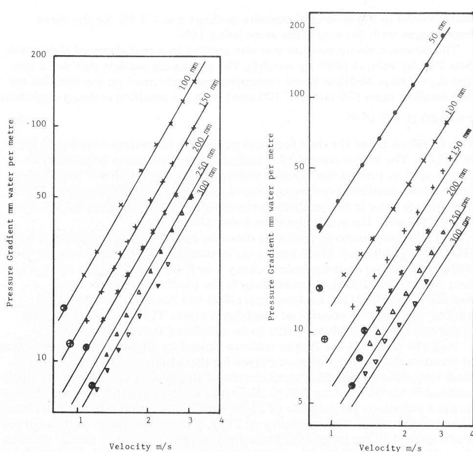
Velocity m/s Velocity m/s Fig.1. Comparison between predicted (full lines) and experimental pressure gradient • Iron ore concentrate slurry, do = 40м, C = 24%. Fig.2. Comparison between predicted (full lines) and experimental pressure gradient • Coal slurry, do = 190 м, C = 32%.

J= 5228 D-1.18 V1.77 (7) where J is in mm of water per m of pipe length; D is in mm; and V is in m/sec. This equation fitted the data for these two pipes with an average correlation error of + 2%. The exponents of V and D in this equation indicate near Newtonian behaviour. The full lines on Fig. 1 show the predicted pressure gradient for all pipe sizes using this equation. Excluding the data where a

stationary bed of particles was present, indicated by the ringed points, the

Page 6

56

average error in the predicted pressure gradient was ‡ 6.4% for the three largest pipes with the maximum error being 14%. The Bowen scale-up method was also applied to a coal slurry of concentration 32% by volume (39% by weight). The maximum particle size was 2 mm and do = 190 u. Multiple linear regression was performed on the data for the two smallest pipes (50 mm and 100 mm) with the resulting scale-up equation: J= 4160 D-1.23 y1.57 (8) This equation fitted the data for these pipes with an average correlation error of + 2.3%. The low exponent of V indicates non-Newtonian behaviour. Eq. 8 can be used to predict the pressure gradient in any pipe size and the comparison between predicted and experimental pressure gradient is shown in Fig.2.

was + 7.2% with the maximum error being 13%. The average error in the predicted pressure gradient for the four largest pipes

The maximum scale-up factor on diameter in the above examples is 3 to 1 (100 mm to 300 mm). When scaling-up to considerably larger diameters than 300 mm involving scale-up factors of say 8 or 9 any scatter in the pilot-plant

data will cause a degree of uncertainty in the predicted pressure drop.

Kenchington (1972) has analysed this effect and has extended Bowen's method by using the concept of confidence limits. This method allows the upper and lower confidence limits to be calculated for each pipe size. - It can be seen that the Bowen scale-up procedure allows accurate prediction of pressure drop in large-diameter pipes for these homogeneous type slurries. Most long-distance pipelines carry slurries of this type. For example the slurry pumped in the 84 km long Savage River iron ore pipeline in Tasmania, Australia has a maximum particle size of 150 u which means that it is finer and hence more homogeneous than the slurry of Fig.1. The longest slurry pipeline in the world is the 430 km long Black Mesa pipeline carrying coal of similar particle size as the slurry of Fig.2. The Bowen scale-up method would be applicable to both these slurries.

SCALE-UP PROCEDURES FOR FLOW OF HETEROGENEOUS SLURRIES

For short-distance pipelines it may be more economical to pump slurries of coarser size, with the consequent higher pressure drops, than to reduce the particle size. Such a case is the iron sand slurry pumped by Waipipi Iron Sands Limited near Waverley, New Zealand. This sand has a maximum particle size of 350 u with 50% greater than 150 u. These heterogeneous type slurries behave differently from the homogeneous slurries and the previous scale-up method cannot be used. The different flow behaviour is illustrated in Fig.3, which shows the behaviour of particles. The heterogeneous slurries no longer show a linear relationship three different slurries all at the same concentration but with different size between log J and log V. At sufficiently high velocities they do behave in a homogeneous manner but these velocities are usually to high for practical

Page 7

57

Heterogeneous

Semi-

LOG J Heterogene

D-

Homogeneous WATER

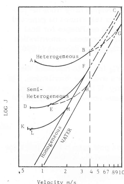
67 8910 Velocity m/s Fig.3. Schematic illustration of the behaviour of the three types of slurries.

applications (say greater than 4 m/sec). As the velocity is decreased the pressure drop curves above that of the homogeneous type. If the velocity is further decreased a minimum pressure drop is reached at a velocity close to the deposit velocity. For a slurry having finer particles than this heterogeneous slurry but not so fine as to behave in a homogeneous manner, the curve labelled "semi-heterogeneous" would apply. This slurry will behave as a homogeneous slurry at velocities attainable in practice say 3 to 4 m/sec but will behave in a settling manner at lower velocities. As a rough criteria for particles of s.g. = 2.65 a semi-heterogeneous slurry would be one having particles of between about 100 and 500 u. A fully heterogeneous slurry would be one having particles greater than 500 u. There have been many correlations proposed for these heterogeneous type slurries some of which are discussed by Thomas and Flint (1974). Most of these correlations relate the incremental increase in pressure drop above that for water flowing at the same velocity. For example, the Durand correlation (Durand, 1953):

Jw gD(S - 1) (9) where J and Jw are the pressure gradients for slurry and water, respectively; C is the delivered volumetric concentration; S' is the specific gravity of the solids; Ca is the drag coefficient of the average sized particles; and K is a constant.

Page 8

58

This equation allows prediction of the slurry pressure drop from the properties (Ca) of the average sized particles. However this cannot be expected to yield accurate results and could not be used with confidence for final design purposes. For instance the assumed linearity between concentration and the increase in pressure drop has been questioned by Babcock (1968) and found not to apply in all cases. Also it is not entirely clear which is the best Ca to use to represent the average properties of the particles when there is a wide size distribution. For these reasons pipe-loop tests are usually necessary. If these are run with a slurry of the same size distribution and at the same concentration as will be pumped in the full size pipe, eq. 9 reduces to: J-Jw = K, Jw D1.5 (10) V3 The uncertainties of the effects of C and Ca have now been sidestepped since these quantities have been absorbed into the constant K1. K, will be determined by pipe-loop tests and eq. 10 can be used simply as a scale-up law. Now from eq. 4 for a homogeneous Newtonian fluid (water): Jw = A VisD-1.2 (11) so that eq. 10 becomes: J- Jw = K, V-1.2 Do.3 (12) i.e., if the increase in pressure drop of the slurry above that for water flowing at the same velocity is plotted against velocity on log log paper it should plot as a straight line of slope - 1.2. Different pipe diameters should be correlated by Do.3. This correlation has been tested for a great number of materials and pipe sizes and is generally accepted as describing the behaviour of these coarse heterogeneous slurries, although slight variations in the exponents of V and D have been proposed by some authors. The recommended scale-up procedure for coarse heterogeneous slurries is therefore as follows: - (1) Plot the results of the pipe loop tests on log-log paper as (J- J..) versus velocity. (2) If they plot as a straight line of slope -1.2 then eq. 12 probably applies although the exponent of D should be checked by tests on different sized pipes. (3) Once the exponents and the value of the constant K2 are determined this equation can then be used as a scale-up law. - When testing extremely coarse slurries, the delivered concentration may vary considerably over the velocity range tested and K, in eq. 12 will not be constant. For such slurries it may be preferable to plot (J - Jw)/C versus velocity. The possibility that (J - Jw) is not directly proportional to concentration is not of great importance since the range of concentration change due to the change in velocity wili be relatively small. Over such a small concentration range (J - J.) will be directly proportional to concentration for all prac-

Page 9

59

tical purposes. However, use of (J- Jw)/C instead of (J - Jw) should be avoided unless necessary, since there are invariably large errors involved in the measurement of C which may introduce unnecessary scatter.

THE BEHAVIOUR OF SEMI-HETEROGENEOUS SLURRIES

Shown on Fig.4 are the results of tests performed on a sand slurry at a concentration of 24% by volume having a particle size distribution such that 50% of the particles are less than 180 u. In this case the experimental points follow a slope of -1.2 at low velocities but at higher velocities they curve away and follow a positive slope. Obviously eq. 12 cannot be used to scale-up this slurry. Zandi and Govatos (1967) recognised this change in behaviour for these relatively fine slurries. They proposed two equations similar to eq. 9 but having an exponent of -1.93 in the low velocity region and -0.35 in the high velocity region. If used as scale-up laws these equations will reduce to equations similar to (12) but with different exponents, i.e.:

J-Jw = K V-2.06 D 0.73 (13)

and:

J-Jw = K V11 D-0.85 (14)

100 90 80 70 60

50

40

metre

im water

_ 3 OPE-2.06 SLOPE*

10

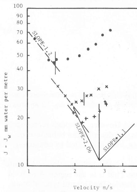
Velocity m/s Fig.4. Experimental results for a sand slurry, do = 180 u, C = 24%, illustrating the behaviour of semi-heterogeneous slurries and allowing comparison with the method of Zandi and Govatos. •, D = 50 mm; x, D = 100 mm; +, D = 150 mm.

Page 10

60 They proposed that the demarcation between the above two equations occurred at:

- = 10 (15) • gD(S - 1) For the 180 -u sand (Cd = 9.71) this gives: V = 1.61 m/sec for D = 50 mm; V = 2.28 m/sec for D = 100 mm; V = 2.79 m/sec for D = 150 mm. Comparing these with Fig.4 it can be seen that although eq. 15 predicts velocity for the larger pipe sizes. Any error in prediction of this velocity will the change in slope fairly accurately for the 50-mm pipe, it overpredicts the cause large errors in pressure-drop prediction, as is illustrated by the full lines drawn for D = 150 mm on Fig. 4 These data do not support the use of the higher exponent of V (-2.06) in eq. 13. As shown by the dashed lines in Fig. 4 an exponent of -1.2 as predicted by equation (12) fits this data better. Neither do these data support the use of a positive exponent of D in eq. 13. To correlate these results a negative exponent of D is required. Zandi and Govatos also proposed that all results below a certain velocity were to be discarded as no longer being in the heterogeneous flow regime so that eq. 13 no longer applied. Their criteria for VVCa < 40 (16) CDg(S - 1) For the 180 -u sand at C = 0.24 this gives: V = 1.58 for D = 50 mm V = 2.23 for D = 100 mm

V = 2.74 for D = 150 mm Applying these to Fig. 4, it can be seen that this criteria is over conservative

and rejects data in the low-velocity region which still follows eq. 13 approxi-

that the Durand equation (eq. 9 or 12) does not describe the behaviour of It is obvious from the above that Zandi and Govatos, although recognising

semi-heterogeneous slurries at high velocities, have also failed to adequately describe the behaviour.

uate scale-up for the heterogeneous slurries. That is in the region A to B or leturning to Fig.3 it has been shown how the Durand equation allows ade

the top clue show to emin to the low elucily ree a pe eat

to higher velocities (E to F). Zandi and Govatos attempted to describe this

region by fitting a straight line of slope +1.1 to the plotted data of (J- Jw) versus V. However reflection on this issue will reveal that the data in the high-

Page 11

61

velocity region of Fig. 4 rather than being of constant slope, must actually be continuously changing slope with increasing velocity. This must be so because at sufficiently high velocities (greater than 4 m/sec on Fig.3) these semi-hete-

rogeneous slurries behave as single-phase homogeneous Newtonian fluids. For

such a fluid: J= K Vis D-1.2 (see eq. 4) (17) But: Jw = Kw VI.s D-1.2 (18) J=(K-Kw+Kw) V1.s D-1.2 (19) and so: J-Jw=(K-Kw) Vs D-1.2 = K, V1.8 D-1.2 (20) Eq. 20 indicates that with these semi-heterogeneous slurries at velocities above 4 m/sec on Fig.3, (J - Ju) must be proportional to V 1.8. This illustrates the basic weakness of the method of Zandi and Govatos in that it attempts to fit two straight lines to the data of Fig. 4 when in actual fact they must follow curves of changing slope. To get the whole range of slurries into perspective, refer once again to Fig.3. With coarse, heterogeneous slurries the Durand equation describes the flow from A to B. These slurries are not normally pumped at higher velocities so that the behaviour above 4 m/sec say is of no consequence. However, if they were pumped at these higher velocities the pressure drop would follow the curve B to C, although the Durand equation would predict behaviour B to G since it states that J - Jw is proportional to V-1.2 so that J must tend to Jw as the velocity increases. As the particle size is reduced, the curve labelled as "semi-heterogeneous" will apply. With such a slurry, the velocity range (D to E) over which the Durand-type equation holds is reduced and the region E to F which Zandi and Govatos tried to describe becomes of practical significance. Once again if the Durand equation is applied to this latter region it would underestimate the pressure drop (E to H). With further reduction in particle size (say slightly less than the 180 u of Fig.4), the slurry would behave as indicated by the lower curve of Fig.3 (K, L, M). The velocity range (K to L) over which the Durand equation applies is now negligible and over most of the velocity range of interest the slurry is in the annoying region (L to M) in which no scale-up procedure has yet been suggested. The method of M.E. Charles Charles (1970) recognised these limitations of the previous correlations and proposed an equation which allowed a smooth transition between the region where the Durand equation applies and the high-velocity region where a slurry behaves as a single-phase fluid. He proposed the equation:

Page 12

62 J- Jw V2 -1.5 C Jw = KI gD(S - 1) VCa + K2(S - 1) (21)

which for a particular slurry at a particular concentration can be written as:

J- Jw = K3 V-1.2 D0.3 + K, V1.8 D- 1.2 (22)

He suggested a value of K1 = 120 and K2 = 1. For the 180 -u sand in the 50-mm pipe this gives the uppermost curve on Fig.5. The dotted points represent the experimental results. It can be seen that although the actual value of the pressure drop prediction is too high, the shape of the curve describes the experimental trends much better than the two straight lines of Zandi and Govatos. At low velocities the second term of eq. 22 becomes insignificant and the function becomes a straight line of slope -1.2, i.e., the Durand equation. At high velocities the first term of eg. 22 becomes insig-

nificant and the function becomes a straight line of slope +1.80, i.e., homo-

geneous flow. With suitable adjustment of the constants eg., putting K1 = 80 and K2 = 0.70 the equation can be made to fit the data reasonably well as is shown by the lower full line of Fig.5. It is apparent that eq. 22 describes the variation with velocity quite successfully. However, the positive exponent of D in the first term does not correlate the data for different pipe diameters

150

100

metre 100 -

• 90%

20

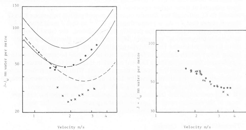
Velocity m/s Velocity m/s Fig.5. Experimental results for a sand slurry, dso = 180 u, C = 24%, allowing comparison with the method of Charles. - •, D = 50 mm; x, D = 100 mm. Fig.6. Experimental results for a sand slurry, do = 480 u, C = 12%. •, D = 50 mm; x, D = 100 mm.

Page 13

63

as was mentioned previously and is illustrated by the dashed curve in Fig.5 which is the predicted curve for D = 100 mm using eq. 22. Correlation of different diameters would require a negative exponent of D in the first term of eq. 22.

The method of Vocadlo and Charles Vocadlo and Charles (1972) approached the problem in a different way but arrived at an equation similar to eq. 22 except for slightly different values of the exponents in the first term. They proposed the equation: Wo 0.2 Pm 0.8

J= KC(S - 1) V + Jw (23)

where K is a constant; Wo is the particle settling velocity; Mm and uw are the viscosities of the mixture and water, respectively; Pm and ow are the densities of the mixture and water, respectively. The second term of this equation represents the homogeneous pressure drop and is of the same order as the [1 + C(S- 1)]J, or pm/p Jw used by Charles in eq. 21. For a particular slurry at a certain concentration eq. 23 can be written as:

J-Jw = K, V-1 + K2 V1.8 D-1.2 (24)

The equation is similar to eq. 22 differing only in the exponents of V and D in the first term. In the discussion on the previous method it was illustrated how Charles's use of a positive exponent of D in the first term of eq. 22 did not correlate the data from different pipe diameters. A more negative exponent was required. In view of this, eq. 24 would be expected to give better correlation of different diameters although a negative exponent of D is really required. Vocadlo and Charles only tested eq. 23 against results from one pipe diameter, so they did not investigate this diameter dependence.

RECOMMENDED SCALE-UP PROCEDURE FOR SEMI-HETEROGENEOUS SLURRIES

It is obvious that equations of the form of eq. 22 and 24 best describe the flow of semi-heterogeneous slurries. They have the advantage over the method of Zandi and Govatos in that they do not require separation into different flow regimes, since they provide for a continuous transition from the high velocity homogeneous flow regime to the low-velocity heterogeneous flow regime. As a result of examining a considerable amount of data it is thought that the exponent of V in the first term of these two equations is closer to -1.2 than -1.0. This means that eq. 22 is more applicable than eq. 24. Eq. 22 also has the advantage of being in agreement with the Durand equation for coarse

Page 14

64 heterogeneous slurries (where the second term of eq. 22 is negligible). However, although eq. 22 describes the variation with velocity quite successfully, in order to correlate the data for the different pipe diameters of Figs. 4 and 5 the exponent of D in the first term is required to be negative rather than positive. On the other hand, for coarse heterogeneous slurries the exponent of D is known to be positive. Apparently the value of the exponent of D in the first term of eq. 22 is dependent on the particle size of the slurry. For coarse particles it is positive but as the particle size is progressively reduced, the exponent is reduced towards zero and eventually becomes negative. This means that for an intermediate particle size the exponent of D would be neither positive nor negative but would be close to zero. Fig.6 shows results for a sand slurry of particle size 480 u at a concentration of 12% by volume. It can be seen that for such an intermediate particle size the exponent of D in the first term would indeed need to be close to zero to correlate the data. The value of the exponent of D is obviously going to depend on the particular slurry and will need to be determined from pipe-loop tests in two or more different sized pipes. The recommended scale-up equation for semiheterogeneous slurries is therefore:

J-Jw= K,V-12D6 + K, V1.8 D-1.2 (25)

where K1, K2 and b need to be determined from pipe-loop tests for a particular slurry at a particular concentration. Since Jw = Kw D-1.2 V 1.8, eq. 25 can be written as:

J= K, D' V-1.2 + K, D-1.2 V 1.8 (26) -

Eg. 26 could be used equally as well for scale-up in place of eg. 25, K1, 6 and K3 needing to be determined from pipe-loop tests. However, the advantage of using eq. 25 is that by examining the shape of log-log plots of - (J- Jw) versus V the slurry can be immediately classified and the degree of heterogeneity can be ascertained. The method of scale-up using eq. 25 will now be illustrated using the same data as in Figs. 4 and 5 for the 50-mm and 100-mm pipes. This data pertains to a 180 -u sand having a narrow size distribution, all particles between 60 and 100 mesh. Concentration is 24% by volume (45% by weight). Data points pertaining to situations where either a sliding or stationary bed of particles had been observed were rejected and the remaining points used to obtain the constants K1, b and K2 in eq. 25. Because this equation is non-linear in these parameters, multiple linear regression can not be applied. Instead an estimate of these parameters was obtained using the technique of non-linear least curve and all data points is minimised. A standard function minimisation subsquares whereby the sum of the squares of the errors between the fitted routine using the Simplex method was employed. - The result of this analysis was K, = 309, b = -0.44 and Kz = 792, i.e.:

J-Jw = 309 D 0.44 V 1.2 + 792D-1.2 V1.8 (27)

Page 15

65

This equation fitted the data for the 50-mm and 100-mm pipes (12 data points) with an average error of = 2.3%.

Fig. 7 allows comparison between predicted values of (J - Jw) obtained

80 40

60 30

mm water per metre 100 150mm mm water per metre

20 200, 1 - J 10

250 300

10

Velocity m/s

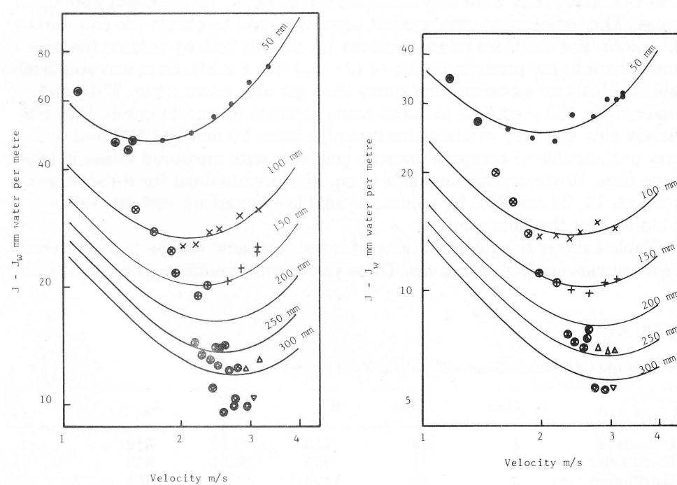
Velocity m/s Fig. 7. Comparison between predicted (full lines) and experimental values of (J - Jw). Sand slurry, do = 180 u, C = 24% •, D = 50 mm; x, D = 100 mm; +, D = 150 mm; *, D = 200 mm; 4, D = 250 mm; v, D = 300 mm. Fig.8. Comparison between predicted (full lines) and experimental values of (J - Jw). Sand slurry, dso = 180 u, C = 12%. •, D = 50 mm; x, D = 100 mm; +, D = 150 mm; *, D = 200 mm; 4, D = 250 mm; v, D = 300 mm.

Page 16

66

the data for the 50 mm and 100 mm pipes was used to obtain the constants in eq. 25. The resulting equation was:

J- Jw = 265 D-0.51 V-1.2 + 311 D-1.2 V 1.8 (28)

This equation fitted the 15 data points for these two pipes with an average error of ‡ 3.4%. Eq. 28 was then used to predict the value of (J - Jw) for the four larger pipe diameters. These predicted curves are shown as full lines on Fig.8. Agreement between predicted and experimental values is seen to be excellent, the average error in (J - Jw) for the four largest pipes being ‡ 2.8% with the maximum error being ‡ 6.1%. These are equivalent to an average error of + 0.6% and a maximum error of + 1.3% in the predicted pressure gradient. The method was also applied to a different sand slurry. This sand had the same dso value (180 u) as the above sand but had a wide size distribution with particles as large as 1.5 mm present and 25% of the particles less than 50 u. For this slurry data were only available for 100-mm, 150-mm and 250-mm pipes. The data for the two smallest pipes was used to obtain the constants in eq. 25. For the three concentrations 15, 20 and 24% by volume the maximum error in the predicted value of (J - Jw) was ‡ 8.5%. Data was also available for tests on a coarser sand slurry than the above two sands. This sand had a dso = 480 u with all particles being between 30 and 50 mesh. Unfortu- nately data was only available for two pipe sizes, 50 mm and 100 mm so it was not possible to compare pressure gradients with measured values in larger pipe sizes. However, the consiants in eq. 25 were obtained for three concentrations 12, 24 and 30% by volume to enable comparison with the values obtained for the finer sands. Table I shows the values obtained for the constants for the three different

sands at various concentrations. These values were obtained using data from -

TABLE I

Values obtained for constants K,, b and K, in eq. 25 Case Conc. 180-u sand 12 283 -0.53 319 Narrow size 2 24 582 -0.61 859 distribution 36 1476 -0.62 1454

-

180-u sand 15 440 -0.49 410 Wide size 20 579 -0.53 527 distribution 24 102 -0.17 693 480-u sand 12 58.9 +0.19 228

24 1050 -0.27 415 9 30 2310 -0.41 1200

Page 17

67

all pipes. For cases 1 and 2 there was data available from six pipes, cases

Some general trends evident from Table I are: (1) The finer the sand the more negative the value of b as was discussed previously. (2) Two slurries having the same value of dso but differing size distributions have different values of b. The 180 - u sand with the wide size distribution generally has a less negative value of b than the 180 -u sand with the narrow size distribution. (3) Generally the value of 6 is seen to become more negative with increasing concentration as would be expected. It has been shown how eq. 25 can be used as a scale-up equation for semiheterogeneous slurries. For the limited range of slurries tested it allows accurate prediction of the pressure gradient. Eq. 25 is largely empirical and it is certainly not suggested that it is theoretically rigorous. However it has been shown to work successfully for the slurries tested and it is reasonable to assume that it will also apply for other types of slurries. Whether or not this is the case can only be decided when adequate data from tests in a larger number of pipe sizes becomes available.

SEMI-HETEROGENEOUS SLURRIES HAVING NON-NEWTONIAN PROPERTIES

If a slurry has a very wide particle size distribution such that very fine particles are present along with some quite coarse particles, it may exhibit heterogeneous behaviour at low velocities but behave in a non-Newtonian homogeneous fashion at higher velocities. For such a slurry eq. 25 cannot be applied because it assumes that the slurry behaves in a Newtonian fashion at high velocities, i.e., at high velocities J= K, D-1.2 V 1.8 (c.f. eq. 4) For a non-Newtonian slurry eq. 6 applies. This means that the exponents of V and D in the second term of eq. 25 are no longer fixed at 1.8 and -1.2 respectively but need to be determined from pipe-loop tests. The scale-up equation for such slurries would therefore need to be of the form:

J=K,D'V-12+K2 V*D (29)

and the five constants K1, b, Kz, x and y would need to be determined.

Page 18

68

SUMMARY OF SCALE-UP PROCEDURE

Simple scale-up procedures have been proposed for all classes of slurries. The method is outlined below. (1) Pipe-loop tests are performed on the slurry at the desired concentration in a number of different diameter pipes and the results plotted on log-log paper as pressure gradient versus velocity. (2) If the result is a straight line for each pipe size then the slurry is behaving as a homogeneous slurry and the Bowen scale-up procedure can be (3) If the result is not a straight line then the slurry is behaving as a heterogeneous slurry. To decide whether it is behaving as a fully heterogeneous slurry or as a semi-heterogeneous slurry, it is necessary to plot the data as (J - Jw) versus velocity, on log-log paper. If the result is a straight line of negative slope (around -1.2) then the slurry is behaving as a fully heterogeneous slurry and eq. 12 can be used to scale-up to larger pipe sizes. (4) If instead of a continuous straight line of negative slope, there is a change in slope from negative to positive as the velocity is increased then the slurry can be classed as semi-heterogeneous. In this case it is recommended that eq. 25 be applied.

ACKNOWLEDGEMENTS

The author thanks M.D. Research Company Pty Ltd. for permission to publish this paper. All experimental data used in this paper was obtained from reports published between March 1973 to January 1974 by the Saskatchewan

Research Council of Canada entitled "Experimental Studies on Solids Pipe- -

lining in Canadian Commodities" and carried out for the Canadian Transport Commission and the Transportation Development Agency.

REFERENCES

Babcock, H.A., 1968. Heterogeneous flow of heterogeneous solids. Int. Symp. on Solid Liquid Flow in Pipes, Univ of Penn., Philadelphia. Symp. Proc. available in book-form as Advances in Solid-Liquid Flow in Pipes and its Application, Pergamon, London, Bowen, R.L., Jr., 1961. Series of articles in: Chem. Eng., June 12, p. 243; June 26, p. 127; - July 10, p. 147; July 24, p. 143; August 7, p. 129; August 21, p. 119. Charles, M.E., 1970. Transport of solids by pipeline. 1st Int. Conf. on the Hydr. Transp. of Solids in Pipes (organised by Br. Hydromech. Res. Assoc.), Univ. of Warwick, England, Pap. A3. cheng, D.C.H., 1970. A design procedure for pipeline flow of non-Newtonian dispersed systems. Ist Int. Conf. on the Hydr. Transp. of Solids in Pipes, Univ of Warwick England, Pap. J5. Dodge, D.W. and Metzner, A.B., 1959. Turbulent flow of non-Newtonian systems.

AIChE J., 5: 189-204.

Page 19

69

Durand, R., 1953. Basic relationships of the transportation of solids in pipes - experimental research. Proc. Minn. Int. Hydr. Conv., Int. Assoc. for Hydr. Res., pp. 89-103. Hanks, R.W. and Dadia, B.H., 1971. Theoretical analysis of the turbulent flow of non- Newtonian slurries in pipes. AIChE J., 17: 554-557. Harris, J. and Quader, A.K.M.A., 1971. Design procedures for pipelines transporting non- Newtonian fluids and solid-liquid systems. Pipes and Pipelines, 16 (4/5): 307—311. Kemblowski, Z. and Kolodziejski, J., 1973. Flow resistances of non-Newtonian fluids in

transitional and turbulent flow. Int. Chem. Eng., 13: 265—279.

Kenchington, J.M., 1972. The design of large pipelines for cement slurries. 2nd Int. Conf. on the Hyd:. Transp. of Solids in Pipes. Univ. of Warwick, England, Pap. e4. Kenchington, J.M., 1974. The prediction of pressure drop in slurry pipelines. Multiphase Phase-Flow Symposium (organised jointly by IChE and IME), Univ. of Strathelyde, Glasgow. Metzner, A.B. and Reed, J.C., 1955. Flow of non-Newtonian fluids - correlation of laminar, transition, and turbulent flow regions. AIChE J., 1: 434—440. Thomas, A.D. and Flint, L.R., 1974. Pressure drop prediction for flow of solid-liquid mixtures in horizontal pipes. Proc. 5th Australasian Conf. on Hydr. and Fluid Mech., Univ. of Canterbury, N.Z., 2: 111-118. Vocadlo, J.J. and Charles, M.E., 1972. Prediction of pressure gradient for the horizontal turbulent flow of slurries. 2nd Int. Conf. on the Hydr. Transp. of Solids in Pipes, (organised by Br. Hydromech. Res. Assoc.), Univ of Warwick, England, Pap. C1. Zandi, I. and Govatos, G., 1967. Heterogeneous flow of solids in pipelines. ASCE Proc. Hydrol. Div., 93(HY3): 145-147.