This HTML edition contains selectable text extracted from the original PDF. Layout-aware OCR was used to recover reading order, figures and equations; minor recognition errors may remain. Consult the PDF for the authoritative layout, figures and equations.

Reprint
of Paper published in
CHEMICAL ENGINEERING IN AUSTRALIA
THE INSTITUTION OF ENGINEERS, AUSTRALIA
A Rational Design Philosophy for Long Distance Slurry Pipelines.
A.D. THOMAS
SUMMARY Various types of slurries ranging from ones with very coarse particles to very fine particles are discussed. It is shown how pressure drop limitations dictate that all long distance slurries have quite fine particles. The differences between typical tailings line slurries in mineral processing plants and the true long distance slurry is discussed and it is shown how the stability of a slurry on shutdown of the pipeline and its ability to be restarted is perhaps the most important requirement for a long distance slurry. It is argued that the stability of a slurry depends on the yield stress of the slurry being sufficiently high to support the largest particles and a simple theory is developed relating these two variables. This requirement and the limitations on maximum economic pressure drop and velocity dictate the available size distribution limits for long distance slurries. Finally economic optimisation of the operating velocity, solids concentration and solids throughput is discussed with the aid of a typical example.
1 INTRODUCTION
The hydraulic transport of solids in pipelines is not new having been used for short distance transport in the mining industry for over a hundred years. In the last decade a few long distance (up to 440 km) pipelines have been built (see Table 1) and there is increasing interest being shown in this alternative transport means.
Because long distance pipelines are relatively new the published information relating to the hydraulic design criteria and methods is scarce and generally vague about details. The majority of research effort and publications have tended to be concerned with the types of slurries which have traditionally been pumped i.e., those pumped in the short distance applications and this information is of little help in the design of a long distance pipeline.
It will be shown here how certain unique requirements of long distance slurry pipelines dictate the design methods used. These same requirements also dictate the solids concentration and particle sizes which can be pumped and the pumping velocity. A discussion of these and the variables shows how the available range for them is limited. This explains why, for a particular commodity, the solids concentration, particle size and pumping velocity of long distance slurries does not vary much from installation to installation.
2 NOTATION
- C solids concentration by volume unless otherwise stated
- D internal pipe diameter
- d particle diameter or mesh size
- F force
- g gravitational acceleration, 9.81
- K constant in equation A2
- DP/L pressure gradient
- Q volume flow rate
- V mean velocity in pipe
- ppl plastic viscosity
- pm density of solids-liquid mixture
- pp density of solid particles
- extrapolated yield stress
- static yield stress
3 HYDRAULIC BEHAVIOUR OF SLURRIES
The behaviour of different types of slurries in horizontal pipe flow is best illustrated by considering a graph of pressure gradient versus mean pipe velocity as in Figure 1 which shows the behaviour of slurries having the same concentration but different particle size in two pipe sizes. Four types can be distinguished (see Thomas (1976) according to the different hydraulic behaviour.
3.1 Type 1 Slurry
This is a typical "settling" slurry having relatively coarse particles. Examples are gravel or coarse sand. These are often described as heterogeneous slurries because of the distinct vertical concentration gradient which exists at velocities near the deposit conditions. At sufficiently high velocities they will flow as pseudo-homogeneous slurries as shown by the straight line portion of the graph. The deposit velocity, defined here as the velocity below which a stationary bed of solids begins to accumulate on the bottom of the pipe, is crucial to design as it is generally desirable to operate above this velocity. For these types of slurries Durand (1953) has shown that the deposit velocity varies as the square root of pipe diameter. This means that the operating velocity becomes very large for large diameter pipes with consequent high pressure gradients. The pressure gradient of these slurries can be estimated using the Durand equation (Durand (1953)).
3.2 Type 2 Slurry
As the particle size is reduced the pseudo-homogeneous portion of the curve extends to lower velocities and the slurry can be termed "moderately settling" or "semi-heterogeneous". For sand, typical median particle sizes might lie between 100 and 500 microns. Thomas (1976) has shown how the pressure gradient of these slurries cannot be scaled up by use of the Durand equation and has suggested an alternative approach. It has further been shown (Thomas (1975)) that for these slurries
* Dr. Thomas is Senior Research Engineer, M.D. Research Company, North Ryde, NSW (Paper H1001 submitted 10 December 1976)
TABLE 1.
SOME LONG DISTANCE SLURRY LINES
| Location | Material | S.G. | Length (km) | Pipe Diameter (mm) | Max. Particle Size (mm) | *Particle Size Limit (mm) | Reference |
|---|---|---|---|---|---|---|---|
| 1 Savage River | Magnetite | 5.0 | 85 | 225 | 0.104 | 0.30 | McDermott et al (1969) |
| 2 Bougainville | Copper Concentrates | 4.3 | 27 | 150 | 0.208 | 0.40 | Piercy (1976) |
| 3 West Irian | Copper Concentrates | 4.3 | 110 | 100 | 0.149 | 0.40 | McNamara (1976) |
| 4 Arizona(Black Mesa) | Coal | 1.4 | 437 | 450 | 2.38 | 3.0 | Wasp (1969) |
| 5 Ohio | Coal | 1.4 | 173 | 250 | 1.41 | 3.0 | Halvorsen (1976) |
| 6 England | Limestone | 2.7 | 112 | 250 | 0.59 | 1.75 | Schriek et al (1973/1) |
| 7 Japan | Copper Tailings | 2.7 | 65 | 200 | 0.208 | 0.70 | Couratin (1969) |
| 8 Turkey | Copper Concentrates | 4.3 | 64 | 125 | 0.149 | 0.40 | Noyan et al (1974) |
| 9 Washington | Limestone | 2.7 | 67 | 200 | 0.295 | 1.75 | Schriek et al (1973/1) |
| 10 Brazil | Iron ore | 5.0 | 403 | 500 | - | 0.30 | Anonymous (1975) |
*Calculated as per Section 6.
Note numbers 6 and 9 flow in laminar flow regime
Number 10 is not yet operating
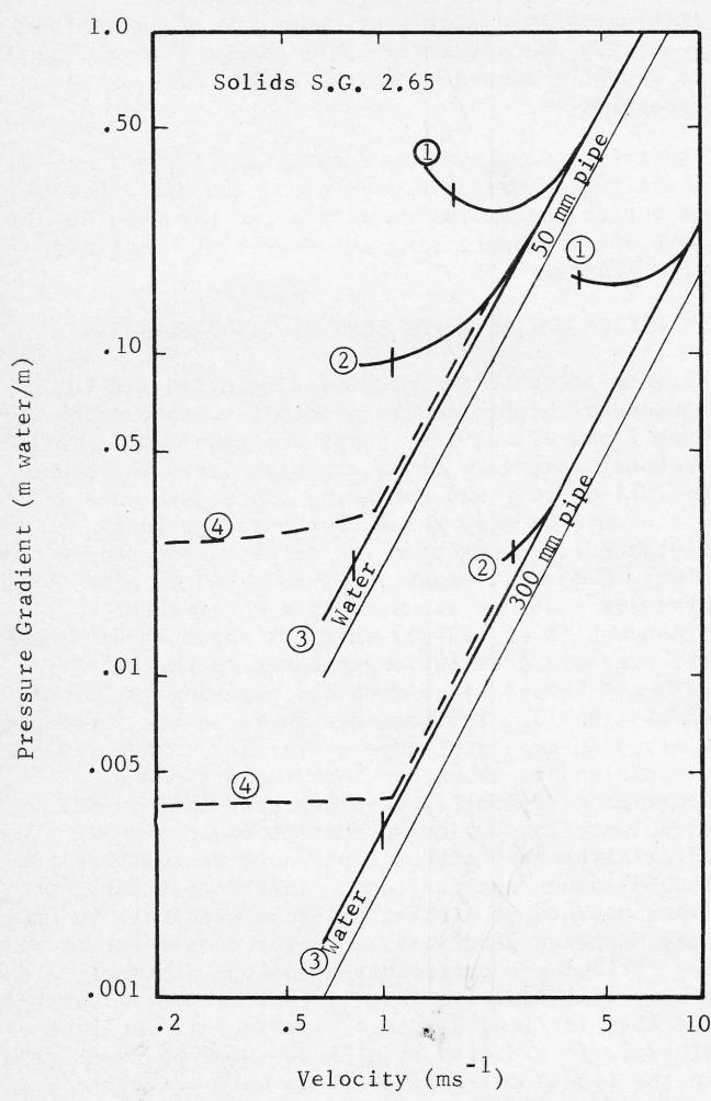
Figure 1. Typical behaviour of different types of slurries
the accuracy of the prediction using the Durand equation depends on the pipe size under consideration. For small pipe sizes (less than about 25 mm) the Durand equation will underpredict while for large pipe sizes (above about 100 mm) the Durand
equation will overpredict. For pipe sizes in the range 25 to 100 mm, where most of the research work is performed, the Durand equation can adequately predict the pressure gradient.
The deposit velocity for these "moderately settling" slurries is less than for the coarser "settling" slurries but is still proportional to . Thus high operating velocities are needed in large pipes. The examples of such slurries are sand mining and dredging applications and some coarser tailings. The iron sand slurry ship loading schemes at Waipipi (Thompson et al (1972)) and Taharoa (Raudkivi (1975)) in latter Zealand are velocities required in the 300 mm pipes are around 5 m/s with the consequent high pressure gradients and high wear rates.
3.3 Type 3 Slurry
As the particle size because is further reduced eventually pseudo-homogeneous behaviour is maintained right down to the deposit velocity as illustrated in Figure 1. For these slurries the deposit velocity is not only lower than for slurries 1 and 2 but is also less dependent on pipe size. Probably the best method available for predicting the deposit velocity is due to D.G. Thomas (1961). He gives an equation from which it can be shown that the deposit velocity is roughly proportional to . This
work was based on experiments on flocculated thorium oxide and kaolin slurries in pipes from 25 to 100 mm. Experimental data on iron ore slurries (Schriek et al (1973/2) and coal slurries (Schriek et al (1973/3)) in pipe sizes from 50 to 300 mm shows a similar dependence of deposit velocity on pipe diameter, as does unpublished data obtained by the author on a number of different slurries in pipe sizes from 19 to 105 mm. This means that even for very large diameter pipes the deposit velocity and hence the operating velocity can be fairly low.
any non-Newtonian effects are present they are relatively insignificant. This means that for design purposes the pressure gradient may be estimated using a Newtonian fluid approach using either the measured viscosity of the slurry or else the calculated viscosity along the lines suggested by Vocado and Charles (1972). An even simpler approach which is extensively used in industry is to simply multiply the water only pressure gradient by the ratio of the density of the slurry to that of water. This latter approach is of course the basis of the slurry pump engineer's measurement of pressure drop in "head of slurry".
Typical examples of type 3 slurries are the usual tailings slurries pumped anywhere from a few hundred metres to 10 or 15 km. Pumping velocities for such slurries are generally around 1 to 2 m/s.
Although these slurries flow in a homogeneous manner at all velocities above the deposit velocity they are termed pseudo-homogeneous because if the flow is stopped they will quickly settle out, the coarsest particles reaching the bottom first and the finest last, to form a bed of solids on the bottom of the pipe.
It can perhaps be noted here that the pressure gradient prediction method presented by Wasp et al (1968) is an attempt to provide a single equation for types 1, 2 and 3 slurries. Their method therefore allows for a smooth reduction in pressure drop as the particle size is reduced and the slurry changes from a type 1 to a type 3.
3.4 Type 4 Slurry
As the particle size is further reduced to the particles are colloidal in proportion behaviour of the slurry if flow is suddenly stopped changes. With these slurries no settling of particles occurs, or if it does, the particles settle (or compact) en masse forming a homogeneous but more concentrated slurry with clear water above. The completely non-settling type of slurry will be referred to as a fully stable slurry while the latter type, where settling occurs but with no particle segregation, will be referred to as a pseudo-stable slurry. Both are defined as type 4 slurries. Such slurries, if flowing under laminar conditions, can be described by non-Newtonian rheological models which are discussed in numerous textbooks e.g. Govier and Aziz (1972). They will be modelled as a Bingham plastic. Typical behaviour of a fully stable slurry would be as shown in Figure 1. For a pseudo-stable slurry laminar flow is not always possible, especially in larger pipe sizes. Thus the fact that a slurry is pseudo-stable, if flow is suddenly stopped does not necessarily mean that laminar flow is possible. This matter will be further discussed later.
Under turbulent flow conditions the behaviour of type 4 slurries will closely parallel the type 3 slurries but will generally exhibit a slightly higher pressure drop because of their more viscous nature.
There is a vast amount of literature published concerning pressure drop prediction of non-Newtonian homogeneous slurries, see for example the book by Govier and Aziz (1972) and a recent distinguish between fully stable and pseudo-stable slurries but is in fact only applicable to the former. Unfortunately, as will be recognized later, the most
suitable long distance slurries are often the pseudo-stable variety.
4 EFFECT OF PARTICLE SIZE DISTRIBUTION ON HYDRAULIC BEHAVIOUR
When considering the different types of slurries it should be noted that not only is the median ( ) particle size important in determining slurry behaviour but also the particle size distribution. For essentially mono-sized particles of sand of S.G. 2.65 typical ranges of particle size might be as follows:
| Type 1 | mm |
| Type 2 | mm |
| Type 3 | mm |
| Type 4 | mm |
With the more usually encountered slurries having wide size distributions with particles perhaps from sub-micron to mm or cm size no typical values can be given given the degree of homogeneity, or conversely heterogeneity, will depend on the proportion of micron size particles, the maximum flocculation. For example, a flocculated slurry of wide size distribution could exhibit all four types of behaviour depending on the concentration, changing from a type 1 slurry at low concentrations to a type 4 slurry at high concentrations. Alternatively a slurry of wide size distribution at a certain concentration could change from a type 1 to a type 4 depending on the degree of flocculation.
The method developed by Wasp et al (1970) which classifies slurries according to the distribution of solids concentration within the pipe may be of some use in quantifying the degree of homogeneity of a slurry.
5 DESIGN CRITERIA FOR LONG DISTANCE SLURRIES
Because of the high velocities required and the consequent high pressure gradients required pumping type 1 and 2 slurries, pumps are when pumped at more frequent intervals along the pipeline. The higher overall capital and operating costs then make it uneconomic. To pump these slurries over long distances. For example the Waipipi iron sands slurry pumped at about 5 ms -1 in a 300 mm pipe has a pressure gradient around .075 m water/metre (Thompson et al (1972)) which is about three times the pressure gradient experienced in the smaller (230 mm) Savage River iron ore pipeline (McDermott et al (1969)). For long distances we are therefore limited to type 3 or type 4 slurries. The previous discussion has shown how both these types of slurries have similar pressure gradients in the turbulent flow regime so that it would seem at first sight that either type would be suitable for long distance applications. Indeed most tailings lines operate at similar pressure gradients to the long distance pipelines. However consideration of the following requirements. Of a long distance slurry will indicate that in fact the only slurry suitable for long distance pipelines is the type 4 slurry. In addition it will be shown how even within the type 4 category there is only a limited range of slurries which are economically suitable.
The major design requirements for a long distance slurry are:
- (a) It must be capable of being stopped for at least a few days and restarted with the pipeline full of slurry.
- (b) Even the coarsest particles must not deposit
out at the normal operating velocity for fear of a slow build up causing a blockage.
(c) The velocity should not exceed about
since, as noted by Wasp (1969), this velocity has been found to be about the economic maximum with single phase fluids such as with oil pipelines. Above this velocity the high pressure gradients causes capital and running costs to rapidly become prohibitive. In any case at velocities much above this wear due to abrasion could become increasingly serious.
These three requirements will now be discussed in detail.
5.1 Restart Capability
That the slurry must be capable of being restarted after stopping is obvious even though such situations may never be envisaged in normal operation. It is often general practice to fill the line with water before any planned long periods of shutdown but the possibility must be allowed for that an unplanned shutdown could occur. If a type 3 slurry is stopped flowing the solids will quickly settle out, the coarsest particles reaching the bottom first and the finest last. Thus a bed of solids will be formed filling perhaps 40 or 50% of the pipe cross section. In a horizontal pipe this bed should present no problem since once flow is started the water flowing in the top section should progressively scour the bed away. In sloping sections of the pipeline the situation is different. The possibility explicit that a bed of particles may slide down the slope and block up the whole pipe cross section at a "valley" section. Another possibility is that the same blockage could arise from flow effect as discussed by Shook (1974). If such a blockage does occur starting of the pipeline will require that this plug be moved. Streat and Televantos (1976) have shown that it is possible to start such plugs and indeed pump continuously at such high concentrations but the pressure gradient required is very high. For closely graded sand they measured and predicted pressure gradients of the order of 1 m water/m regardless of pipe size which is some 50 to 100 times higher than the typical tailings line pressure gradient. The situation with wide size distributions is likely to be worse since they tend to pack tighter than narrow size distributions. Clearly it would not require a very long length of plugged line before the start up pressure required was beyond the capability of the pumps.
In spite of this it is common knowledge that many tailings lines, the solids of which settle out to form a bed on shutdown, can usually easily be restarted. However every now and again these tailings lines do block up but because of their short lengths and because they are usually situated above the ground it is not too difficult to locate the blockage and clear the line. In other words it is far better to accept the possibility of the line blocking up occasionally than to go to the additional cost of grinding the tailings finer just to achieve a type 4 slurry for transportation. (The very concept of tailings disposal requires that the solids settle out at the disposal area anyway).
With a long distance slurry pipeline perhaps some hundreds of kilometres in length and with the pipeline buried under the ground even the remotest possibility that a blockage can occur must be avoided. For this reason all long distance slurry
pipelines should ideally employ type 4 slurries which have been previously described as those which do not settle out to form a bed of solids when stopped.
As discussed previously a type 4 slurry can be either fully stable or pseudo-stable. Obviously a fully stable slurry which remains completely homogeneous even after days of standing will not present any start up problems. A pseudo-stable slurry can also be restarted as has been inferred by Wasp (1969) when he refers to fast or slow settling slurries being permissible as long as the material settles homogeneously.
To determine whether a slurry will be stable (fully or pseudo) a simple stability criterion has been developed (see Appendix). It is based on the assumption that the coarsest particles will not settle providing the upwards force due to the slurry yield stress exceeds the gravitational force. For a particular yield stress (either static or extrapolated see Appendix) this criterion enables the maximum stable particle size to be calculated. Conversely for a given maximum particle size it permits calculation of the required yield stress. The yield stress of a slurry is largely due to the interaction between colloid or near colloid size particles. This necessarily means that the slurry must have a wide size distribution. A typical distribution for a coal slurry might be 5 to 10% greater than 1 mm ranging down to 15 to 30% less than 50 microns.
The importance of the yield stress in determining slurry stability has been clearly illustrated by tests by the author (Thomas (1975)) on a finely ground quartz slurry. This was a ball mill product which, as produced, was largely dispersed (de-flocculated) and possessed virtually no yield stress. If allowed to settle this slurry quickly formed a solid bed of particles which were packed so hard that the bed could oftenonly be removed by a considerable amount of chipping with a hammer and chisel. However when the pH of the slurry was lowered a yield stress and became a completely stable slurry which did not settle and remained fluid for weeks.
The yield stress which type 4 slurries possess must be overcome to restart a stopped pipeline. For a completely homogeneous type 4 slurry which does not settle at all on shutdown it is the yield stress of the slurry as pumped which must be overcome to restart the pipeline. For a pseudo stable type 4 slurry which compacts on shutdown there is the possibility that this compacted slurry will plug in the low "valley" sections of the pipeline either by sliding or by density currents. To restart the pipeline it is necessary to overcome the yield stress of this compacted slurry in the plugged sections. This compacted slurry, because of its higher solids concentration will have a higher yield stress than the slurry as pumped.
In horizontal lengths of pipe the clear water layer on top would be expected to begin moving first since it requires no yield stress to initiate motion. As it moves it would pick up the compacted portion and dilute it and so eventually as long as the yield stress of the pumped slurry was overcome the line would start moving again.
The possibility exists, however remote, that upon shutdown, all of the compacted slurry moves to the lower "valley" sections of the pipeline so that the whole pipeline consists of plugs of compacted
slurry separated by plugs of clear water. The water filled sections require no pressure to initiate motion but the compacted slurry sections require that sufficient pressure be applied to everywhere exceed the yield stress in these sections. As an example suppose a coal slurry is pumped at 40% volume concentration and that this slurry has an extrapolated yield stress of 3 Pa. Suppose that on shutdown this slurry slowly compacts down to a homogeneous slurry occupying only 80% of the previous volume i.e., there is a clear water layer on top occupying 20% of the volume. Suppose that the yield stress of this 50% concentration compacted slurry is 8 Pa. The worst possible situation occurs if 80% of the line length consists of plugs of compacted slurry requiring 8 Pa stress to start flow and 20% of the line is clear water requiring no stress to start flow. i.e., In the plugged sections the shear stress at the wall of the pipe on commencement of flow, is given by
so that the total pressure required before flow will commence is given by
Providing this pump pressure is available the pipeline should be able to restart under any conditions. This would suggest that the grade limitations placed on the earlier lines (for instance Savage River was limited to a maximum of 10% grade - McDermot et al (1969)) may be unnecessarily conservative. Possibly this was later realised because it was designed by E. Wasp (Wasp, (1969)) that "We put a slope limitation of somewhere between 10 and 15%, but not always. We are building one line now without a slope limitation". Further evidence is provided by McNamara (1976). Further the copper concentrate pipeline in Irian Jaya. He states that this line was designed to a maximum grade of 18% but that during construction several problems of 26% and 28% were built. No start-up problems are mentioned.
Obviously the more stable the slurry the less likely are steep grades going to be of importance. A further consideration is that with a pseudo-stable slurry which compacts on shutdown the degree of compaction may be influenced by the weight of slurry above so that in long steeply sloping sections the concentration of the compacted slurry at the bottom could be greater than when tested in a bench experiment. This would need to be investigated for each particular slurry.
The laminar flow curves of the type 4 slurry in Figure 1 illustrate the tendency for the laminar velocity in large pipes i.e., to become dependent only on the yield stress and independent of the plastic viscosity of the Bingham model. Thus for laminar flow curves in large pipe sizes the laminar flow curves can be drawn as horizontal lines of constant pressure gradient. a
The requirement that the slurry be stable on shutdown means that a certain minimum yield stress is required which depends on the maximum particle size. Thus the dashed lines on Figure 2 show permissible idealised laminar flow curves to ensure a stable slurry. Consideration of the second and third design requirements means that an upper limit is placed on the yield stress.
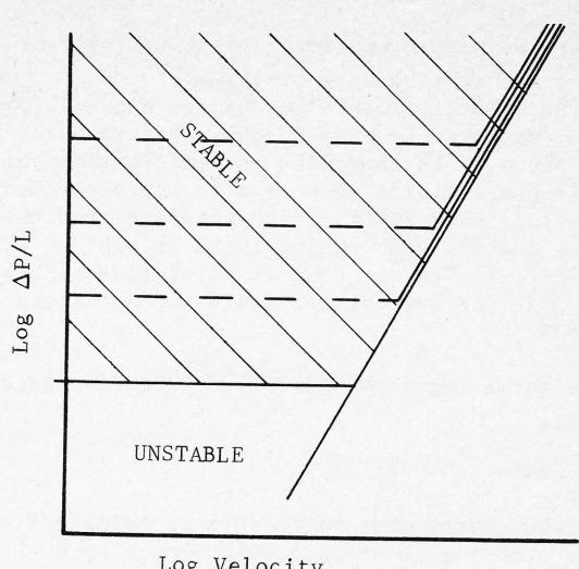
Figure 2. Effects of stability considerations on available operating region.
5.2 No Deposition of Particles During Operation
This is the second design requirement. The stability criteria given by equations A6 and A7 in the Appendix should ensure either a stable or pseudo-stable slurry on sudden shutdown. However, whereas a fully stable slurry can be operated in the laminar flow regime, a pseudo-stable slurry often cannot. This can be explained by the breakdown of the floc structure under conditions of laminar shear. It is generally agreed (see Michaels & Bolger (1962/2)) that the floc structure is broken during laminar shear, indeed this explains the reduction in apparent viscosity with increasing shear rate of a Bingham plastic. The broken floc structure is less able to support the coarsest particles thus causing deposition. This is more likely to happen in large pipe sizes because, in small pipe sizes, an apparent bridging effect (Michaels & Bolger (1962/1)) increases the strength of the floc structure. Figure 3 provides evidence
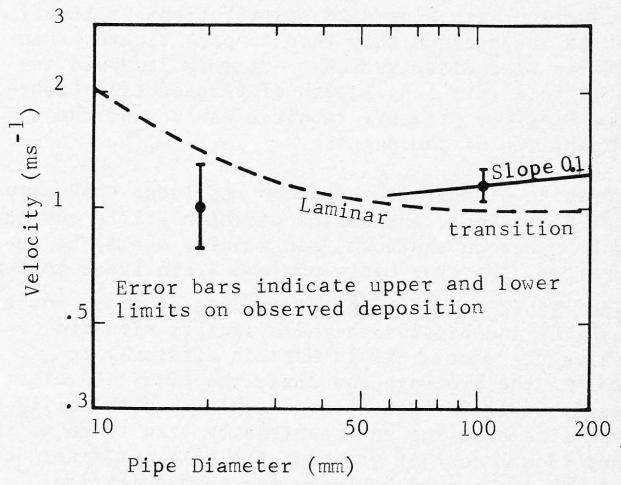
Figure 3. Variation of deposit velocity with pipe diameter for a fast compacting slurry.
of this phenomenon. It shows experimental results obtained by the author for a loam slurry in two pipe sizes, 19 and 105 mm. The loam consisted of about 20% clay with the remaining sand having a top size of 0.82 mm. In the smaller pipe laminar/
turbulent transition was observed at (visually through transparent without section). At steady laminar flow was observed. At a bed of solids formed. Thus the critical deposit velocity lay somewhere between and , well below the laminar/turbulent transition velocity. The same slurry, at the same concentration, in the larger pipe behaved differently. In this case deposition occurred under turbulent flow conditions. By scaling up from the laminar flow results obtained in the smaller pipe (see Bowen (1961/1) it was estimated that the laminar/turbulent transition velocity in the large pipe was about , although laminar flow conditions could not be realised.
The slurry of Figure 3 illustrates typical pseudo-stable slurry behaviour which has been observed by the author with a number of different slurries. If turbulent flow is suddenly stopped the coarsest particles remain in suspension. Sustained laminar flow is only possible in small pipe sizes and in turbulent flow at velocities above the laminar/turbulent transition velocity. For pipe sizes large enough for deposition to occur under conditions of turbulent flow the deposit velocity will vary as as for a type 3 slurry.
The author knows of no method of predicting a priori whether deposition will occur under laminar or turbulent flow conditions. For rapidly settling pseudo-stable slurries it would therefore seem necessary to perform pipe loop tests in increasingly larger pipe sizes until deposition occurs in the turbulent regime. Once this size pipe is reached the deposit velocity in larger pipe sizes can be obtained by assuming it varies as as for a type 3 slurry.
5.3 The Velocity Should Not Exceed About for Economic Reasons
Operation above is generally uneconomic due to the rapid increase in pressure. This places an upper limit on the yield stress. Because of the uncertainty associated with whether or not laminar flow is possible it is generally desirable that the pipeline be operated in the turbulent regime. To ensure that operation is fully within the turbulent regime and to allow for possible variation in slurry properties and inaccuracies in prediction methods the transition velocity should not exceed about . Note that this, then allows a safety margin of above to allow for the possibility of deposition occurring in the turbulent regime as discussed above. For Figure 3 only approaches the usual operating velocity range of to for pipe diameters greater than about so for pipes smaller than this there would be no problem if design were based on the laminar transition velocity. In short, as long as the slurry does not compact very fast on shutdown (say within a few minutes), the design can be based on the laminar transition velocity. For a fast compacting pseudo stable slurry especially in large pipe tips it would be wise to perform small diameter loop tests to check whether deposition does occur in the turbulent regime, and then scale-up by assuming the deposit velocity varies as .
The allowable limits on are now shown in Figure 4. Note that by plotting versus Figure 4 is applicable to all large pipe sizes. The upper limit dictated by the maximum limit on transition velocity represents a maximum yield
stress, , of about an iron or slurry ranging about for a coal slurry. Both these depend slightly on the pipe diameter. Note that the turbulent pressure gradient is not greatly dependent on the yield stress although it will differ for different solids S.G.'s. As an example, Piercy (1976) has stated that the yield stress for the Bougainville copper concentrate slurry (solids S.G. 4.3) is maintained below a maximum limit of which is in agreement with the above stated limits. The lower limit for stability depends on the maximum particle size.
If the slurry is completely stable, operation within the laminar regime is feasible. For example the Rugby limestone pipeline in England operates under laminar conditions. (Shriek et al (1973/1)) In this case the same economic limits on maximum pressure gradient apply so that the upper limit can be raised as shown in Figure 4. This limit would be about 2.5 times the previous limits i.e.,
for iron or down to for coal.
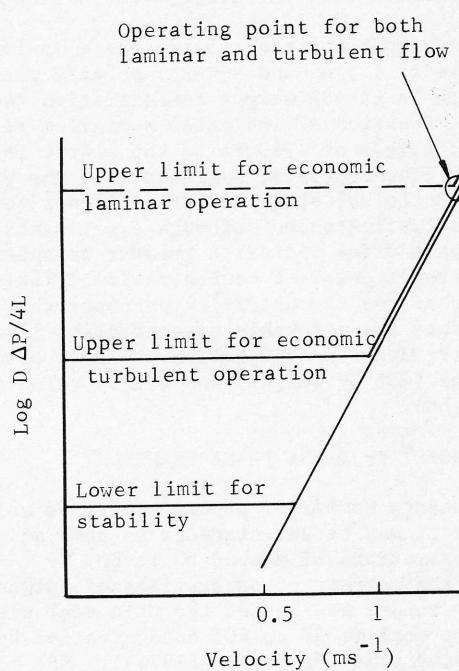
Figure 4. Yield stress limits for laminar and turbulent flow operation.
6. CONSEQUENT LIMITS ON MAXIMUM PARTICLE SIZE
Considering only turbulently flowing slurries, for they are by far the most common, the upper limits of for iron or and 3 for coal mean that the maximum possible particle size for a stable slurry is (from equation A7 of the Appendix) about for iron or ranging up to about for coal. Of course a slurry can operate with maximum particle sizes considerably less than these limits and may have to be prevented deposition during operation but there is a limit to how fine the particles can be ground for pipelining due to the rapidly increasing yield stress and hence pressure gradient as size is reduced due to increasing colloidal effects. For example the work of Friend and Hunter (1971) suggests that the yield stress increases as the square of the reciprocal of the particle size for colloidal size particles.
Table 1 gives some details of nine existing long distance slurry pipelines together with the maximum economic particle size as calculated above. In every case the maximum particle size is less than
the calculated maximum limit the actual values ranging from one fifth to four fifths of the limit. The economic limits on maximum particle size for long distance slurries would appear to lie between 20% and 100% of the value given by equation A7 using equal to 4.5 Pa for iron ore ranging down to 3.0 Pa for coal.
7 LIMITS ON CONCENTRATION
Most reports on slurry pipeline installations specify upper and lower limits to the permissible range of concentration. For example Halvorsen (1976) mentions the limits on the Ohio coal pipeline as being 50% and 44% by weight. The reasons for these limits should now be obvious and following the reasoning outlined above it is possible to calculate the allowable limits for any particular slurry.
The upper limit is set by the necessity to stay below the maximum economic yield stress (3 Pa for coal, 4.5 Pa for iron ore). The lower limit is set by the requirement that the slurry remain stable.
As an example suppose a coal slurry has a maximum particle size of 1.5 mm and an extrapolated yield stress of 2.6 Pa at 48% weight concentration (40% by volume). Equation A7 indicates a minimum required yield stress of 1.62 Pa so the slurry is stable. D.G. Thomas (1963) suggests that the yield stress of a colloidal slurry is proportional to volume concentration cubed although experiments by the author have often indicated greater dependence up to the seventh power of concentration. Taking the third power for demonstration purposes this would mean that the allowable concentration limits for the slurry under consideration would be between 34% by volume (43% by weight) and 42% by volume (50% by weight).
8 THE CONCEPT OF DENSE PHASE TRANSPORT
There have been a number of papers published which suggest that it may be advantageous to pump at higher concentrations of around 50 to 60% by volume than the current concentrations of between 25 to 45% by volume and indeed the Ohio coal pipeline did pump coal at 58 to 60% concentration by weight for some time (Halvorsen (1976)). The most notable papers are those due to Bantin and Streat (1970) and Elliott & Glidden (1970). The first of these was concerned with coarse sand (around 0.7 mm) of narrow size 1 mm. They found that particles less than about 0.1 mm. They were not that could be pumped at concentrations above 55%. Streat and Bantin (1972) and Streat and Televantos (1976) have further pursued this line. However, as mentioned previously, the pressure gradients in this type of flow are extremely high, some 50 to 100 times usual practice, and so it would only be of use for very short distances. Another line of approach was taken by Elliott and Glidden where they found that by pumping a wide size distribution coal slurry containing appreciable colloidal size material at concentrations above 50% coal particles up to 12.5 mm could be transported under laminar flow and the slurry was stable and could be stopped and restarted. A7 in the now easily explained. Equations A6 and A7 in the Appendix indicate that provided the yield stress is made sufficiently high any top size particle can be supported and so the slurry made stable. But as discussed previously there is a limit to the maximum yield stress due to economic considerations of pumping pressures. It was been shown that limits of about 3 Pa ( ) for turbulent flow operation or about 7.5 Pa for a completely stable coal slurry operating in laminar flow are
reasonable for long distance applications. A study of Elliott & Glidden's paper will reveal that the extrapolated yield stress ensuring a stable slurry with the 12.5 mm top size was around 10 Pa. (at 59% concentration by weight). This is in close agreement with the 11 Pa limit indicated by equation A7. Note, however, that it is higher than the 7.5 Pa economic limit and so may prove uneconomic for long distances. Similarly for a 3.2 mm top size they found that a 57.2% by weight concentration was stable ( Pa) while 53% concentration was not stable. The yield stress of the latter is difficult to ascertain but they did state that the yield stress approximately doubled with every 5% increase in concentration by weight. This would suggest a yield stress of about 2.7 Pa. It is remarkable that equation A7 indicates a value of 2.9 required for stability.
Thus it can be seen that slurries of virtually any top size can be made stable providing the yield stress is made large enough. An increase in concentration increase. Alternatively the surface properties of the colloidal particles can be altered by pH changes or by addition of flocculants to increase flocculation and so increase the yield stress. As noted by Elliott & Glidden this latter effect can cause quite dramatic changes in the yield stress. Whether pH or flocculant will affect a slurry depends entirely on the surface chemistry of the slurry and so each slurry needs to be treated individually.
In some cases pH changes or the addition of deflocculants may be needed to decrease the yield stress so that an economic pumping pressure can be obtained.
The main thrust of Elliott & Glidden's paper was concerned with adjustment of particle size distribution to achieve a stable slurry with minimum pressure gradient. There can be little doubt that adjustment of the size distribution to ensure maximum packing density will produce a less viscous slurry with a lower yield stress. But the stability theory presented here suggests that this could then mean that a lower top size will be required if stability is to be maintained.
It is hoped that the concept of dense phase flow can now be seen in proper perspective. Nothing unusual happens when the concentration is increased above 50% by volume. The stability can still be explained by equations A6 and A7. One simply needs to be aware that transportation of coarser particles as a stable slurry is achieved at the expense of higher pressure gradients. For long distance applications this rapidly becomes uneconomic once the maximum particle size exceeds the limits mentioned previously. For short distance applications it may well be warranted.
9. THE DESIGN PROCEDURE
It is now possible to form a design procedure and suggested steps for the design of a long distance slurry pipeline operating in the turbulent flow regime are outlined below:
9.1 Determine Maximum Particle Size
The maximum economic velocity limit and the consequent limit on maximum yield stress of about 4.5 Pa ( ) for iron ore and about 3 Pa for coal immediately requires from equation A7 that the maximum particle size be no greater than about 0.3 mm for iron ore and about 3 mm for coal.
turbulent transition was observed at (visually through transparent viewing section). At steady laminar flow without deposition was observed. At a bed of solids formed. Thus the critical deposit velocity lay somewhere between and , well below the laminar/turbulent transition velocity. The same slurry, at the same concentration, in the larger pipe behaved differently. In this case deposition occurred under turbulent flow conditions. By scaling up from the laminar flow results obtained in the smaller pipe (see Bowen (1961/1) it was estimated that the laminar/turbulent transition velocity in the large pipe was about , although laminar flow conditions could not be realised.
The slurry of Figure 3 illustrates typical pseudo-stable slurry behaviour which has been observed by the author with a number of different slurries. If turbulent flow is suddenly stopped the coarsest particles remain in suspension. Sustained laminar flow is only possible in small pipe sizes and in large pipe deposition occurs under conditions of turbulent flow at velocities above the laminar/turbulent transition velocity. For pipe sizes large enough for deposition to occur under conditions of turbulent flow the deposit velocity will vary as as for a type 3 slurry.
The author knows of no method of predicting a priori whether deposition will occur under laminar or turbulent flow conditions. For rapidly settling pseudo-stable slurries it would therefore seem necessary to perform pipe loop tests in increasingly larger pipe sizes until deposition occurs in the turbulent regime. Once this size pipe is reached the deposit velocity in larger pipe sizes can be obtained by assuming it varies as as for a type 3 slurry.
5.3 The Velocity Should Not Exceed About for Economic Reasons
Operation above is generally uneconomic due to the rapid increase in pressure. This places an upper limit on the yield stress. Because of the uncertainty associated with whether or not laminar flow is possible it is generally desirable that the pipeline be operated in the turbulent regime. To ensure that operation is fully within the turbulent regime and to allow for possible variation in slurry properties and inaccuracies in prediction methods the transition velocity should not exceed about . Note that this then allows a safety margin of above to allow for the possibility of deposition occurring in the turbulent regime as discussed above. For Figure 3 only approaches the usual operating velocity range of to for pipe diameters greater than about so for pipes smaller than this there would be no problem if design were based on the laminar transition velocity. In short, as long as the slurry does not compact very fast on shutdown (say within a few minutes), the design can be based on the laminar transition velocity. For a fast compacting pseudo stable slurry especially in large pipe diameter pipes it would be wise to perform small pipe loop tests to check whether deposition does occur in the turbulent regime, and then scale-up by assuming the deposit velocity varies as .
The allowable limits on are now shown in Figure 4. Note that by plotting versus Figure 4 is applicable to all large pipe sizes. The upper limit dictated by the maximum limit on transition velocity represents a maximum yield
stress, , of about an iron or slurry ranging to about for a coal slurry. Both these depend slightly on the pipe diameter. Note that the turbulent pressure gradient is not greatly dependent on the yield stress although it will differ for different solids S.G.'s. As an example, Piercy (1976) has stated that the yield stress for the Bougainville copper concentrate slurry (solids S.G. 4.3) is maintained below a maximum limit of which is in agreement with the above stated limits. The lower limit for stability depends on the maximum particle size.
If the slurry is completely stable, operation within the laminar regime is feasible. For example the Rugby limestone pipeline in England operates under laminar conditions. (Shriek et al (1973/1) In this case the same economic limits on maximum pressure gradient apply so that the upper limit can be raised as shown in Figure 4. This limit would be about 2.5 times the previous limits i.e.,
for iron or down to for coal.
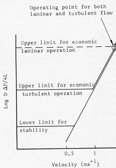
Figure 4. Yield stress limits for laminar and turbulent flow operation.
6. CONSEQUENT LIMITS ON MAXIMUM PARTICLE SIZE
Considering only turbulently flowing slurries, for they are by far the most common, the upper limits of for iron or and 3 for coal mean that the maximum possible particle size for a stable slurry is (from equation A7 of the Appendix) about for iron or ranging up to about for coal. Of course a slurry can operate with maximum particle sizes considerably less than these limits and may have to be premit deposition during operation but there is a limit to how fine the particles can be ground for pipelining due to the rapidly increasing yield stress and hence pressure gradient as size is reduced due to increasing colloidal effects. For example the work of Friend and Hunter (1971) suggests that the yield stress increases as the square of the reciprocal of the particle size for colloidal size particles.
Table 1 gives some details of nine existing long distance slurry pipelines together with the maximum economic particle size as calculated above. In every case the maximum particle size is less than
the calculated maximum limit the actual values ranging from one fifth to four fifths of the limit. The economic limits on maximum particle size for long distance slurries would appear to lie between 20% and 100% of the value given by equation A7 using equal to 4.5 Pa for iron ore ranging down to 3.0 Pa for coal.
7 LIMITS ON CONCENTRATION
Most reports on slurry pipeline installations specify upper and lower limits to the permissible range of concentration. For example Halvorsen (1976) mentions the limits on the Ohio coal pipeline as being 50% and 44% by weight. The reasons for these limits should now be obvious and following the reasoning outlined above it is possible to calculate the allowable limits for any particular slurry.
The upper limit is set by the necessity to stay below the maximum economic yield stress (3 Pa for coal, 4.5 Pa for iron ore). The lower limit is set by the requirement that the slurry remain stable.
As an example suppose a coal slurry has a maximum particle size of 1.5 mm and an extrapolated yield stress of 2.6 Pa at 48% weight concentration (40% by volume). Equation A7 indicates a minimum required yield stress of 1.62 Pa so the slurry is stable. D.G. Thomas (1963) suggests that the yield stress of a colloidal slurry is proportional to volume concentration cubed although experiments by the author have often indicated greater dependence up to the seventh power of concentration. Taking the third power for demonstration purposes this would mean that the allowable concentration limits for the slurry under consideration would be between 34% by weight (43% by weight) and 42% by volume (50% by weight).
8 THE CONCEPT OF DENSE PHASE TRANSPORT
There have been a number of papers published which suggest that it may be advantageous to pump at higher concentrations of around 50 to 60% by volume than the current concentrations of between 25 to 45% by volume and indeed the Ohio coal pipeline did pump coal at 58 to 60% concentration by weight for some time (Halvorsen (1976)). The most notable papers are those due to Bantin and Streat (1970) and Elliott & Glidden (1970). The first of these was concerned with coarse sand (around 0.7 mm) of narrow size 1 mm. They found that particles less than about 0.1 mm. They within that limit could be pumped at concentrations above 55%. Streat and Bantin (1972) and Streat and Televantos (1976) have further pursued this line. However, as mentioned previously, the pressure gradients in this type of flow are extremely high, some 50 to 100 times usual practice, and so it would only be of use for very short distances. Another line of approach was taken by Elliott and Glidden where they found that by pumping a wide size distribution coal slurry containing appreciable colloidal size material at concentrations above 50% coal particles up to 12.5 mm could be transported under laminar flow and the slurry was stable and could be stopped and restarted. This is now applicable indicated. Equations A6 and A7 in the expendix explained that provided the yield stress is made sufficiently high any top size particle can be supported and so the slurry made stable. But as discussed previously there is a consideration of maximum yield stress due to economic considerations of pumping pressures. It was shown that limits of about 3 Pa ( ) for turbulent flow operation or about 7.5 Pa for a completely stable coal slurry operating in laminar flow are
reasonable for long distance applications. A study of Elliott & Glidden's paper will reveal that the extrapolated yield stress ensuring a stable slurry with the 12.5 mm top size was around 10 Pa. (at 59% concentration by weight). This is in close agreement with the 11 Pa limit indicated by equation A7. Note, however that it is higher than the 7.5 Pa economic limit and so may prove uneconomic for long distances. Similarly for a 3.2 mm top size they found that a 57.2% by weight concentration was stable ( Pa) while 53% concentration was not stable. The yield stress of the latter is difficult to ascertain but they did state that the yield stress approximately doubled with every 5% increase in concentration by weight. This would suggest a yield stress of about 2.7 Pa. It is remarkable that equation A7 indicates a value of 2.9 required for stability.
Thus it can be seen that slurries of virtually any top size can be made stable providing the yield stress is made large enough. An increase in yield stress can be achieved most simply by a concentration increase. Alternatively the surface properties of the colloidal particles can be altered by pH changes or by addition of flocculants to increase flocculation and so increase the yield stress. As noted by Elliott & Glidden this latter effect can cause quite dramatic changes in the yield stress. Whether pH or flocculant will affect a slurry depends entirely on the surface chemistry of the slurry and so each slurry needs to be treated individually.
In some cases pH changes or the addition of deflocculants may be needed to decrease the yield stress so that an economic pumping pressure can be obtained.
The main thrust of Elliott & Glidden's paper was concerned with adjustment of particle size distribution to achieve a stable slurry with minimum pressure gradient. There can be little doubt that adjustment of the size distribution to ensure maximum packing density will produce a less viscous slurry with a lower yield stress. But the stability theory presented here suggests that this could then mean that a lower top size will be required if stability is to be maintained.
It is hoped that the concept of dense phase flow can now be seen in proper perspective. Nothing unusual happens when the concentration is increased above 50% by volume. The stability can still be explained by equations A6 and A7. One simply needs to be aware that transportation of coarser particles as a stable slurry is achieved at the expense of higher pressure gradients. For long distance applications this rapidly becomes uneconomic once the maximum particle size exceeds the limits mentioned previously. For short distance applications it may well be warranted.
9. THE DESIGN PROCEDURE
It is now possible to form a design procedure and suggested steps for the design of a long distance slurry pipeline operating in the turbulent flow regime are outlined below:
9.1 Determine Maximum Particle Size
The maximum economic velocity limit and the consequent limit on maximum yield stress of about 4.5 Pa ( ) for iron ore and about 3 Pa for coal immediately requires from equation A7 that the maximum particle size be no greater than about 0.3 mm for iron ore and about 3 mm for coal.
9.2 Perform Settling Tests to Determine Stability.
A sample of the commodity reduced down to a size distribution such that the maximum particle size is less than the above limits can now be made up into a slurry of typical concentration. The usual concentration required to obtain reasonable solids throughput range from 25% by volume for iron ore to 50% for coal. Slurries of about this concentration should be mixed and then allowed to settle for a day or so. If they do not settle, or if they settle into a compacted homogeneous mixture, they are suitable as far as stability is concerned.
9.3 Determine Yield Stress for Start Up Calculation.
The yield stress of these stable or pseudo-stable slurries should be found to be greater than indicated by equations A6 or A7. But they may be much greater than this and indeed might be too high to permit startup after shutdown. If the slurry is completely stable the slurry as is should be tested for yield stress. If the slurry has compacted the top layer of water should be drained off and then only the compacted portion tested. In both cases the measured yield stress must be low enough to ensure that start up is possible. As mentioned previously the relevant yield stress is the extrapolated yield stress and this is best obtained using a tube viscometer. (e.g. Wazer et al (1963)). However a rotational viscometer can be used if it operates at sufficiently high shear rates. Alternatively a rotational viscometer such as the Brookfield instrument can be used to obtain the static yield stress which is explained in the Appendix can then be multiplied by about 5 times to get an approximate value for .
9.4 Obtain Laminar Flow Curve.
Next the laminar flow curve relating pressure gradient to velocity for the pipe sizes of interest needs to be determined so that scale-up by the method of Bowen (1961/1) can be performed. This requires tests on the original mixed slurry which for a pseudo-stable slurry is at a lower concentration than the compacted portion which was tested above for start up purposes. Some pseudo-stable slurries may compact very quickly after obtaining ceases which can make it difficult to assign meaningful results from a rotational viscometer. Such slurries should be tested in a vertical tube viscometer where settling is no problem. Slowly compacting or fully stable slurries can be tested in a rotational viscometer. If the flow curve for the full range of shear rates of interest cannot be obtained this need not be a serious limitation since, as indicated by Figs 2 and 4, for large pipes the flow curve is dependent almost solely on the extrapolated yield stress. If a rotational viscometer is used but does not permit sufficiently higher shear rates to obtain the extrapolated yield stress an approximate value for can be found by multiplying the static yield stress by about 5.
9.5 Obtain Turbulent Flow Curve
The next step is to obtain the turbulent flow curve. This tests or pipe loop tests (scaled up using the Bowen (1961/2 method)). However if these are not available a reasonable estimate can be made by considering the slurry as a Newtonian
fluid having a density equal to the slurry density and a viscosity equal to the Bingham plastic viscosity. Cheng (1970) suggests that this method overpredicts by about 12%.
9.6 Determine Transition and/or Deposit Velocity
The intersection of the laminar and turbulent flow curves gives the transition velocity for the pipe size under consideration. This should be less than about . If this is so the slurry would be suitable for long distance pipelining at about 1.5 to 1.75 . For a fast compacting pseudo-stable slurry in large diameter pipes deposition may occur in the turbulent regime. In such cases pipe loop tests may be desirable.
9.7 Investigate Possible Changes in Slurry Properties.
Upon testing the originally selected size distribution and concentration the slurry may be found to be quite suitable. However more likely it will not be perfect. There are two possibilities:
9.7.1 The slurry may not be stable. If this is the case equations A6 or A7 indicate two alternatives. Either the particle size can be reduced or the yield stress can be increased. This latter option can be achieved by either an increase in concentration or by a change in the surface chemical properties to increase flocculation. The first alternative would be the most sensible since this means that a higher solids throughput can be achieved. The steps 9.3 to 9.6 can then be repeated.
9.7.2 The slurry is stable but the yield stress is too high. This can be reduced by either decreasing the concentration or by possible de-flocculation. The latter option is obviously the most attractive so that solids throughput can be maintained but it may not always be chemically or economically possible.
10. SPECIFIC ENERGY CONSUMPTION AND SOLIDS THROUGHPUT.
For a slurry of any given maximum particle size it has been shown how upper and lower limits can be placed on the allowable concentration. It is of practical importance to have knowledge of the effect that operation at different concentrations has on the specific energy consumption and on the solids throughput.
Figure 5 shows a plot of specific energy (Joules , ) versus solids throughput (tonnes/year) with concentration, volume flow rate (or velocity), and pressure gradient as parameters. This has been prepared for the following design situation.
coal S.G. 1.40
Maximum particle size 1.4 mm
Pipe diameter 450 mm
at
(15 centipoise) at
Both and vary as in the range of interest. Consideration of Figure 5 shows that the available region of operation is bordered:
- (a) to the left by the need for the concentration (and hence the yield stress) to be sufficiently high to ensure stability.
- (b) to the bottom by the need to operate at a
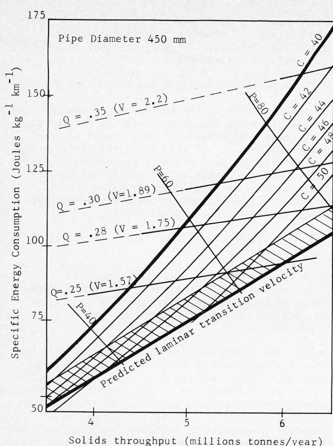
Figure 5. Performance graph for a typical coal slurry.
P = pressure gradient (KPa. km
-1
)
Q = volume flow rate (m
3
. s
-1
)
V = velocity (m. s
-1
)
C = concentration (volume %)
velocity sufficiently above the predicted laminar transition velocity to ensure operation in the turbulent regime. A safety margin of 0.3 ms -1 has been assumed and is represented by the hatched area. (c) to the top by limits on either the maximum economic velocity or the maximum pressure available.
This plot shows that both for a given solids throughput and a given maximum pressure it is more efficient to operate at the highest possible concentration and the lowest possible velocity within the limitations imposed by the above considerations.
11 CONCLUSIONS
It has been shown how the three design considerations of stability on shutdown, avoidance of deposition during operation, and economic limit to maximum velocity and pressure, are considered to available range of particle sizes and concentration suitable for long distance slurry transportation. To aid in the consideration of slurry stability a simple theory has been developed based on the concept of the largest particles being supported by the yield stress of the slurry. The presented design considerations and stability theory result in limits on particle size and slurry properties which are in excellent agreement with all information available to the author concerning existing long distance slurry pipelines.
Using the above concepts a series of design steps are outlined which should serve as a design procedure for long distance slurry pipelines. This can be based entirely on bench scale tests although for
final design and optimisation it would be preferable to have the results of pipe loop tests. Also for pseudo-stable slurries which compact very fast, pipe loop tests may be necessary to determine if deposition occurs in the turbulent regime. This is especially desirable if a very large diameter pipe is being considered. (say in excess of 300 mm diameter).
12 ACKNOWLEDGEMENTS
The author thanks M.D. Research Company Pty. Limited for permission to publish this paper.
13 REFERENCES
ANONYMOUS (1975) New Slurry Pipeline, Mechanical Engineering , October, p. 68.
ANSLEY, R.W. and SMITH, J.N. (1967) Motion of Spherical Particles in a Bingham Plastic. A.I.Ch.E. Journal Vol. 13, pp 1193-1196.
BANTIN, R.A. and STREAT, M. (1970) Dense-Phase Flow of Solids - Water Mixtures in Pipelines. Hydrotransport 1 Conference , Coventry, England, paper G1 British Hydromechanics Research Association.
BOWEN, R.L. (1961/1) Designing Laminar-Flow Systems Chemical Engineering , June 12, pp 243-248
BOWEN, R.L. (1961/2) Designing Turbulent Flow Systems. Chemical Engineering , July 24, pp 143-150
BOARDMAN, G. and WHITMORE, R.L. (1961) The static Measurement of Yield Stress, Laboratory Practice , November, pp 782-785.
CHENG, D.C.H. (1975) Pipeline Design for Non-Newtonian Fluids, The Chemical Engineer , Parts 1 & 2, Sept & Oct.
CHENG, D.C.H. (1970) A Design Procedure for Pipeline Flow of Non-Newtonian Dispersed Systems, Hydrotransport 1 Conference , Coventry, England, paper J5 British Hydromechanics Research Association.
COURATIN, P. (1969) Tailing Disposal, World Mining , May, pp 38-43.
DINA, M.L. (1976) Operating Experiences at the 1580 MW Coal Slurry Fired Mohave Generating Station, First Int. Conference on Slurry Transportation , Columbus, Ohio, Feb. 3rd Slurry Transport Association, Washington, D.C., U.S.A.
DURAND, R. (1953) Basic Relationships of the Transportation of Solids in Pipes - Experimental Research. Proceedings 5th Minneapolis Minesota International Association for Hydraulics Research .
ELLIOT, D.E. and GLIDDEN, B.J. (1970) Hydraulic Transport of Coal at High Concentration. Hydrotransport 1 Conference , Coventry, England, paper G2 British Hydromechanics Research Association.
FRIEND, J.P. and HUNTER, R.J. (1971) Plastic Flow Behaviour of Coagulated Suspensions Treated as a Repetition Phenomenon. J. Colloid and Interface Science Vol. 37, No. 3 pp 548-556.
GAY, E.C., NELSON, P.A. and ARMSTRONG, W.P. (1969) Flow Properties of Suspensions with High Solids Concentration, A.I.Ch.E. Journal , Vol. 15, n 6, November, pp 815-822.
GOVIER, G.W. and AZIZ, K. (1972) The Flow of Complex Mixtures in Pipes , Van Nostrand Reinhold, New York.
HALVORSEN, W.J. (1976) Slurry Pipeline Hydraulics Improved. The Oil and Gas Journal , March 22, 1976, pp 62-66.
MCDERMOTT, W.F., DAVIS, R.A., COWPER, N.T. and
WASP, E.J. (1969) The World's First Long Distance Iron Ore Slurry Pipeline. Mining Engineering , January, pp 86-89.
MCNAMARA, E.J. (1976) Operational Problems with a 69 mile Copper Concentrate Slurry Pipeline. Hydrotransport 4 conference , Banff, Canada, Paper F3, British Hydromechanics Research Association.
MICHAELS, A.S. and BOLGER, J.C. (1962/1) Settling Rates and Sediment Volumes of Flocculated Kaolin Suspensions, Industrial and Engineering Chemistry Fundamentals , Vol. 1, No. 1, Feb., pp 24-33.
MICHAELS, A.S. and Bolger, J.C. (1962/2) The Plastic Flow Behaviour of Flocculated Kaolin Suspensions, Industrial and Engineering Chemistry Fundamentals , Vol. 1, n 3, August, pp 153-162.
NOYAN, K., AKSOY, S., JENSEN, J.H. and WRIGHT, P.B. (1974) The KBI Parallel Pipelines for Sulphide Concentrates. Hydrotransport 3 Conference , Colorado, U.S.A., Paper B2, British Hydromechanics Research Association.
PIERCY, P. (1976) Hydraulic Transport of Copper Concentrate At Bougainville. Transport of Minerals in the Process Industries , Half Day Symposium, Newcastle Chemical Engineering Group, University of Newcastle, July, pp 29-35.
RAUDKIVI, A.J. (1975) Private Communication. Uni. of Auckland, N.Z.
SCHRIEW, W., SMITH, L.G., HAAS, D.B. and HUSBAND, W.H.W. (1973/1) Experimental Studies on Solids pipelining of Canadian Commodities Report II . Experimental studies on Hydraulic Transport of Limestone. Saskatchewan Research Council, Canada.
SHRIEK, W., SMITH, L.G., HAAS, D. and HUSBAND, W.H.W. (1973/2) Experimental Studies on Solids Pipelining of Canadian Commodities Report III . Experimental Studies on the Hydraulic Transport of Iron Ore. Saskatchewan Research Council, Canada.
SHRIEW, W., SMITH, L.G., HAAS, D. and HUSBAND, W.H.W. (1973/3) Experimental Studies on Solids Pipelining of Canadian Commodities Report V . Experimental Studies on the Hydraulic Transport of Coal - Saskatchewan Research Council, Canada.
SHOOK, C.A. (1974) Experimental Studies on Solids Pipelining of Canadian Commodities Report IX . Saskatchewan Research Council, Canada.
STREAT, M. and BANTIN, R.A. (1972) Mechanism of Hydraulic Conveying at High Concentrations in Vertical and Horizontal Pipes. Hydrotransport 2 Conference , Coventry, England, Paper B2, British Hydromechanics Research Association.
STREAT, M and TELEVANTOS, Y. (1976) Pilot Plant Studies of Hydraulic Conveying of Coarse Materials at High Concentration in Pipelines. Hydrotransport 4 Conference , Banff, Canada, Paper F2 British Hydromechanics Research Association.
THOMAS, A.D. (1976) Scale-Up Methods for Pipeline Transport of Slurries. International J. Mineral Processing , Vol. 3 pp 51-69.
THOMAS, A.D. (1975) Unpublished data at M.D. Research Company.
THOMAS, D.G. (1961) Transport Characteristics of Suspensions: II Minimum Transport Velocity for Flocculated Suspensions in Horizontal Pipes. A.I.Ch.E. Journal Vol. 7, No. 3, pp 423-430.
THOMAS, D.G. (1963) Transport Characteristics of Suspensions VII. Relation of Hindered Parameters, Flocculated China clay suspension Archimedes' principle held to within about 2.5% which was insignificant variation compared with the experimental error involved.
THOMPSON, T.L., FREY, R.J., COWPER, N.T. and WASP, E.J. (1972) Slurry Pumps - a survey. Hydrotransport 2 Conference , Coventry, England, Paper H1, British Hydromechanics Research Association.
VOCADLO, J.J. and CHARLES, M.E. (1972) Prediction of Pressure Gradient for the Horizontal Turbulent Flow of Slurries. Hydrotransport 2 Conference , Coventry, England. Paper C1, British Hydromechanics Research Association.
WASP, E.J. (1969) What Slurry Pipelining is all About. Pipeline Engineer , Nov, pp 30-35.
WASP, E.J., AUDE, T.C., SEITER, R.H. and JACQUES, R.B. (1970) Deposition Velocities, Transition Velocities, and Spatial Distribution of Solids in Slurry Pipelines, Hydrotransport 1 Conference , Coventry, England, Paper H4, British Hydromechanics Research Association.
WASP, E.J., AUDE, T.C., SEITER, R.H. and THOMPSON, T.L. (1968) Hetero-Homogeneous Solids on Liquid Flow in Pipes. Int. Symp. on Solid-Liquid Flow in Pipes , Uni. of Penn., Proceedings available in book "Advances in Solid-Liquid Flow in Pipe and its Application", edited by I. Zandi, Pergamon, Oxford (1971).
WAZER, J.R., LYONS, J.W., KIM, K.Y. and COLWELL, R.E. (1963) Viscosity and Flow Measurement - A Laboratory Handbook of Rheology , Wiley, New York.
APPENDIX
Criteria for Stable Slurry
It has been shown that to permit restarting of a stopped pipeline the slurry must be either completely stable even when stopped or if it does settle it must compact with no preferential settling of the coarser particles. This latter case has been termed pseudo-stable. What governs whether a slurry will fit these requirements?
Consider the largest particles in a slurry immediately after shutdown. These particles will fall if the nett gravitational force exceeds the resistance force due to the yield stress of the slurry. This then is the criterion for a slurry to yield stress (either completely or pseudo) - the stress required to support the coarsest particles.
If the stress everywhere on the surface of a sphere of diameter is the resistance force in the vertical direction can be shown to be given by
The exact stress distribution on a sphere immersed in a Bingham plastic is not known so that equation (A1) needs to be replaced by.
To prevent settling of the particle this force must exceed the nett gravitational force acting on the fluid the nett gravitational force is determined by allowing for the buoyancy effect of the fluid as per Archimedes' principle. However in a stable slurry at rest the coarse particles are supported by the plastic yield stress and Archimedes' principle may not be valid for such slurries if the pressure cannot be transmitted hydrostatically. Because of this Ansley & Smith (1967) state that buoyancy should not be allowed for. However Boardman and Whitmore (1961) found that for a flocculated China clay suspension Archimedes' principle held to within about 2.5% which was insignificant variation compared with the experimental error involved.
with flocculated suspensions is perhaps not really surprising. In a flocculated suspension the colloidal size particles are attracted together to form "puffy" flocs. At high concentrations and conditions of low or zero shear rate these flocs cluster together to form an aggregate structure. It is this structure which supports the coarse particles in a stable slurry. However it is conceivable that each large particle might only be supported at two or three points with a fluid layer occupying the particles. Under such conditions Archimedes' principle would be expected to hold, to some degree at any rate. Based on the evidence of Boardman & Whitmore the nett gravitational force has been calculated allowing for the buoyancy effect. (It will be shown later that if buoyancy had not been allowed for the stability theory would be in poor accord with the reported particle sizes of commercial slurries). To prevent settling:
where is the density of the particle and is the density of the mixture. Equating A2 and A3
Ansley and Smith (1967) considered spheres falling in Bingham plastic slurries. They give pertinent data for spheres which fell slowly and another which was supported in a particular slurry. From this K can be found equal to 2.3 so that equation (A4) becomes
This then is the stability criterion. will be the diameter of the largest particle present.
Before applying this equation to pipeline design it is necessary to consider a rheological aspect of slurries. Figure A1 shows an experimentally determined plot of shear stress versus apparent shear rate obtained using a tube viscometer for a coal slurry tested by the author and having a size distribution almost identical to that reported by Dina (1976) for the Black Mesa coal slurry. This can be converted to a plot of shear stress versus true shear rate and this is obtained in Figure A2 along with similar results shown in Figure A3 from a Brookfield rotational viscometer with a cylindrical bob rotating in a very much larger container. If the straight line portion of this plot gives extrapolated yield stress, , which together with the plastic viscosity, provide the Bingham plastic parameters. Thus the Bingham model is seen to fit this slurry for shear rates above about . The full line in Figure A1 is the shear stress versus apparent shear rate relationship calculated according to the Bingham model. At very low shear rates the measured shear stress is seen to be less than the Bingham parameter, , but for pipe sizes and velocities of commercial interest this is immaterial. Note that the yield stress obtained with the Brookfield instrument, termed the static yield stress, , is only 2.6 Pa i.e., about one fifth of . However, similar tests on various pure clay suspensions have given values from the Brookfield instrument almost equal to the values obtained in the tube viscometer. Thus the ratio depends on the properties of the
slurry. In fact it appears to depend on the size distribution of the slurry. A slurry having all colloidal size material such as clay gives values approaching 1 while a slurry such as the above coal slurry having only about 15% colloidal size (less than .01 mm) particles gives values of around 5. Physically this can be explained by assuming the Brookfield instrument measures the yield stress due to the colloidal size particles only whereas the extrapolated yield stress obtained using the tube viscometer depends both on the colloidal effects as well as a purely mechanical component due to any coarse particles present similar to that investigated by Gay et al (1969). In the Brookfield instrument with the bob rotating in a container of effectively infinite diameter the slurry is not constrained and so, possibly helped by centrifugal migration of the coarse particles, the bob only "sees" the colloidal material. In the tube viscometer the slurry is constrained and so the coarse particles contribute to the extrapolated yield stress.
Equation A5 was obtained from the data of Ansley & Smith (1967). They employed tomato sauce (catsup) whose properties were obtained by fitting Bingham's equation to tube viscometer data, i.e., their yield stress is equivalent to here. Tomato sauce would be expected to have few, if any, coarse particles present so that from the above discussion if had been measured using a Brookfield instrument the result would be expected to be approximately equal to . Thus equation A5 can be replaced by
For a slurry consisting almost entirely of colloidal size material with perhaps only a few percent coarse particles, in equation A6 could be replaced by . However in the case of the more usual commercial slurries having a wide size distribution so that if only is available equation A6 can be replaced by
This is only an approximation but in the author's experience is generally between 4 to 6 times for the slurries of commercial type size distribution. It should be noted that is obtained from a true shear rate plot. If the straight line portion of the apparent shear rate (8V/D) plot is extrapolated to zero shear the intercept will be 4 . (dashed line on Figure A1).
Equations (A6) and (A7) therefore provide the required stability criterion. Equation A6 is the preferable one to use if is available. As examples, a typical top size for a coal slurry (coal S.G. 1.4) might be 10 mesh (2.0 mm). For a 40% by volume concentration equations A6 and A7 indicate a minimum required yield stress of or . Piercy (1976) has provided information relating to the Bougainville copper concentrate pipeline. This slurry, solids S.G. 4.3, top size 0.208 mm is pumped at between 55 and 70% concentration by weight. Taking the lower of these values equations A6 and A7 indicate a required minimum yield stress of or . This latter value is remarkably close to the minimum permissible yield stress of 2.1 Pa as stated by Piercy.
It was noted earlier that there is some doubt as to the validity of the buoyancy correction with plastic fluids. However on the basis of the experimental evidence of Boardman & Whitmore (1961) it
was allowed for and the stability criteria expressed in equation A6 and A7 were consequently developed. The limits on maximum particle size, calculated using these equations and the limitations on yield stress discussed in Section 5, can now be compared with the actual maximum particle size of different commercial slurries. Referring to Table 1 the ratio of calculated maximum particle sizes of, for example, coal and magnetite is 10:1 compared to the actual ratio of the Black Mesa coal to the Savage River magnetite of 23:1 or using the Ohio coal 14:1. If the buoyancy correction had not been made these ratio would have been 2.4 and 1.4 respectively. Obviously the values using the
buoyancy correction are much closer to the actual values providing strong evidence that the stability criteria developed here, allowing for the buoyancy correction, is most realistic.
It should be noted that the stability criteria developed here cannot distinguish between a fully stable slurry and pseudo-stable one. To be completely stable and hence capable of being operated under laminar flow conditions a slurry may have to have a yield stress well above that given by equations A6 or A7, especially for operation in large diameter pipes as was discussed in Section 5.2.
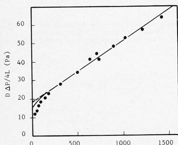
Apparent Shear Rate ( )
Figure A1. Coal slurry test results from tube viscometer. Shear stress versus apparent shear rate.
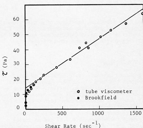
Figure A2. Coal slurry test results from tube viscometer and rotational viscometer. Shear stress versus true shear rate.