Reprint

of a Paper Presented
at a Technical Conference
of

THE INSTITUTION OF ENGINEERS, AUSTRALIA

Particle Size Effects in Turbulent Pipe Flow of Solid-Liquid Suspensions

A. D. THOMAS

Senior Research Engineer, M.D. Research Co., North Ryde

SUMMARY The classic work in the field of hydraulic transport of solids is that due to Durand (1953) but since then numerous workers have pointed out shortcomings of his pressure gradient prediction method. Using carefully selected experimental data the limitations of the Durand approach are revealed. It is found that a mostly neglected parameter, the ratio of particle size $d$ to viscous sub-layer thickness $\delta$ , is of importance. Lack of consideration of this parameter emplains many of the reported discrepancies of the Durand equation. The result is a relatively simple procedure which is shown to be applicable over the whole range of particles sizes and pipe diameters and which can be used to confidently predict the pressure gradient of narrow size distribution suspensions.

1 INTRODUCTION

Figure 1 shows results obtained by the author for two different sands of median particle size of 0.13 mm and 1.20 mm in two different pipe diameters, 18.9 mm and 105 mm. Both sands are of narrow size range, the first having 98% of solids between .070 and .210 mm and the second 98% between 0.60 mm and 2.00 mm and the delivered concentration in both cases is nominally 12% by volume. The exhibited horizontal pipes with suspensions of discrete particles in liquids. The purpose of this paper is to develop a method of predicting such behaviour given the particle size and solids specific gravity.

2 NOTATION

C Volume concentration of solids

• C _d Particle drag coefficient
• D Pipe diameter
• d Particle size
• g gravitational constant
• J pressure gradient of suspension
• J _w Pressure gradient of water flow at same mean velocity as the suspension.
• S specific gravity of solids
• V mean velocity in pipe
• V _c critical velocity below which a sliding bed of particles appears
• V _d critical deposit velocity below which a stationary bed of particles appears
• V* friction velocity for water
• V* _c friction velocity at critical conditions
• W settling velocity of a single particle
• $\delta$ viscous sub-layer thickness for water
  $=5w/(ϵw{V}^{*})$ (See Hinze (1959))
• $\xi$ viscosity defined by equation 8
• $u$ viscosity of suspension defined by equation 5
• $u_w$ viscosity of water
• $e_w$ density of water
• $\rho$ non-dimensional excess pressure gradient defined by equation 2
• $\Psi$ modified Froude number defined by equation 3

• 1 "heterogeneous" portion pertaining to energy required to maintain particles in suspension

• 2 "homogeneous" portion pertaining to energy loss due to particle-particle and particle-fluid interactions.

• 3 THE DURAND EQUATION & $\rho$ VERSUS $\Psi$ PLOTS

Durand (1953) proposed the equation

$$\rho =K{\Psi }^{-1.5}(1)$$

$$\text{where }\rho =\frac{J-J_w}{C{J}_w}(2)$$

$$\text{and }\Psi =\frac{V^2{C}_d}{gD(S-1)}(3)$$

Durand did not give a value for the constant $K$ and it has been variously reported as 81 and 150.

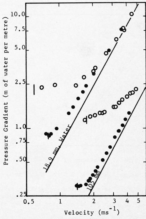
Figure 1 Typical behaviour, Sand C = 12%, $•$ 0.13 mm C 1.20 mm

The data for the two different sands in Figure 1 have been replotted in Figures 2 and 3 using the Durand variables $\varnothing$ and $\Psi$ . Data obtained by the author using a 53.8 mm pipe have also been included. All plots are for a nominal concentration of 12% by volume although the actual concentrations ranged from 7.4% to 13.5% and these were used in each case to calculate $\varnothing$ . In calculating the particle drag co-efficient, $C_d$ , the median particle size was used along with the calculated settling velocity of a sphere of that size in water at that temperature. The resulting values were 0.71 and 13.3 for the 1.2 and 0.13 mm sands respectively.

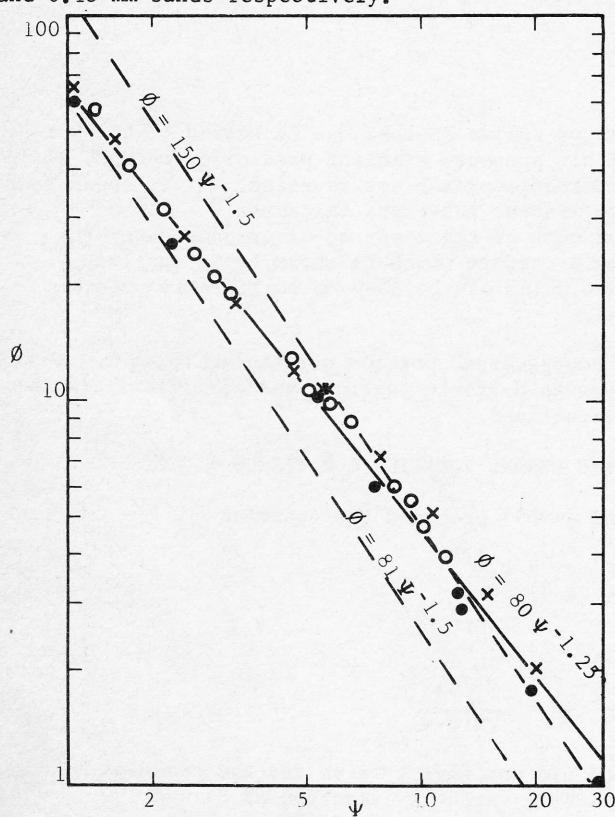
Figure 2 Typical behaviour of coarse (1.2 mm) sand, $C=12\%$

• $D=18.9$ mm, $\times 53.8$ mm, $0105$ mm

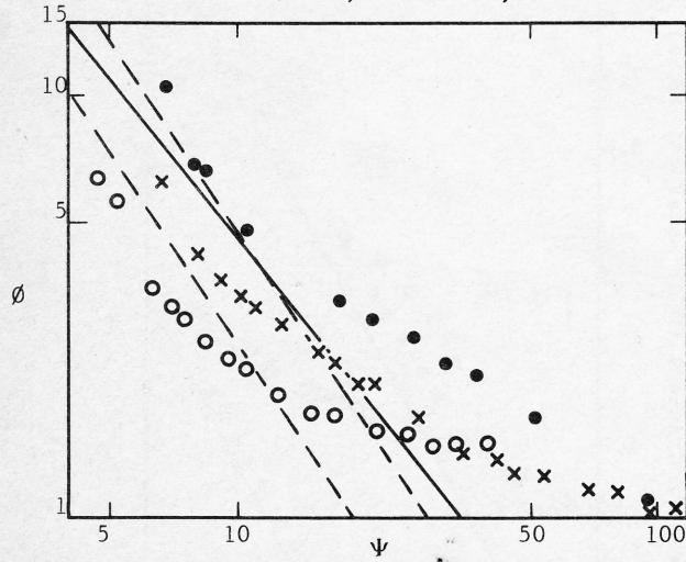
Figure 3 Typical behaviour of fine (0.13 mm) sand, $C=12\%$

• $D=18.9$ mm, $\times 53.8$ mm, $0105$ mm

Figure 2 shows that a definite correlation exists between $\varnothing$ and $\Psi$ for the 1.2 mm sand although the data appear to best fit an equation of lower slope such as

$$\varnothing =80{\Psi }^{-1.25}(4)$$

rather than equation 1. This lower slope has also been noted by Babcock (1968), Hayden and Stelsun (1968) and Toda et al (1969).

Equation 4 appears to adequately correlate the data for the 1.2 mm sand but data on a 0.82 mm sand, not presented here, revealed that the inclusion of the particle drag co-efficient in equation 4 overcompensated for particle size and that in fact for $C_d\lesssim 1$ the pressure gradient is independent of particle size as has been suggested by Newitt et al (1955) and Babcock (1968). This fact immediately explains some of the scatter which has been evident on the $\varnothing$ - $\Psi$ plots of, for example, Zandi & Govatos (1967). However, it is not a major source of scatter, since the inclusion of $C_d$ in equation 4 only causes a relatively small error in $\varnothing$ in the range .

The main source of scatter in the $\varnothing$ - $\Psi$ plots is revealed by considering Figure 3. This shows that for fine particles not only do the data points deviate from a straight line but the paths for different pipe diameters are displaced markedly. The departure from the Durand equation (1967) collected data from numerous sources, some 1450 points in all, and also found that the scatter was greatest at high $\Psi$ values. The change in slope at $\Psi \approx 10$ for fine particles was noted by Zandi and Govatos but the displacement of the curves for different pipe diameters appears to have gone unnoticed except by Thomas (1976). Note that in the low velocity region near the critical velocity the Durand equation underpredicts the pressure gradient for small pipe sizes increasing. This trend is further illustrated by the data of Schriek et al (1973) for 0.175 mm sand in 52 and 315 mm diameter pipes where, at low velocities there is a difference of some 400% in the value of $\varnothing$ for the two pipe sizes for identical $\Psi$ values.

4 FLOW IN HIGH VELOCITY REGION

4.1 Basic Differences between Fine and Coarse Particles

An inspection of Figures 1 and 3 will reveal that the change in slope on the $\varnothing$ - $\Psi$ plot at $\Psi \ge 10$ is related to the paralleling of the pressure gradient to the water line. Inherent in the Durand equation is the assumption that the excess pressure gradient $J_w$ , approaches zero as the velocity increases or in other words the slurry pressure gradient approaches the water only pressure gradient. In Figure 1 the results for the 18.9 mm pipe suggests that this is the case for the coarse sand but not for the fine sand, the data of which appear to parallel the water line. Qualitatively this different behaviour can be explained by the fact that particles smaller than the viscous sub-layer can enter the sub-layer and so raise the effective viscosity in the wall region where (see for example Hinze (1959)) the major part of turbulence generation and direct viscous dissipation occurs. In contrast, coarse particles have little effect on the sub-layer so that the effective viscosity in the wall region will be essentially the same as the viscosity of the fluid medium.

The region of high velocity flow where pseudo homogeneous flow prevails is similar to the flow of suspensions in vertical pipes and to the flow of neutrally buoyant particles. In both these cases

the importance of the ratio of particle size to viscous sub-layer thickness ( $d/\delta$ ) has been recognized (Durand (1953)), Maude & Whitmore (1958), Newitt et al (1961) and Daily & Roberts (1966) and it generally agreed that fine particles produce higher pressure gradients than do coarse particles.

4.2 Assumed Model for High Velocity Flow Regime

The model for the pseudo-homogeneous region can now be outlined. For as a first approximation the pressure gradient can be calculated using the usual friction factor - Reynolds number relationship with the viscosity calculated using any of the suitable equations proposed in the literature, e.g. Thomas (1965).

$$u/u_w=1+2.5C+10.05C^2+\mathrm{.062}\exp \left(\frac{1.875C}{1-1.995C}\right)(5)$$

For coarse particles much larger than the viscous sub-layer the majority of evidence from both vertical fipe flow (Durand (1953), Newitt et al (1961) and Toda et al (1969)) and from the flow of neutrally buoyant particles (Dailey & Roberts (1965)), indicates that the pressure gradient is near the water value. There is very little data for the flow of coarse, settling suspensions at very high velocities in horizontal pipes. One exception is the work of Murphy et al (1955) who suggested the following equation.

$$J_2/J_w=1.07(6)$$

which seems to agree with the data obtained by the author. Using equations 5 and 6 $J_2/J_w$ can now be determined for both very high and very low $d/\delta$ values. Figure 4 shows the resulting values for $C=\mathrm{.12},\mathrm{.20}$ and $\mathrm{.30}$ for particles of S.G. 2.65. Also shown are experimental results obtained by the author and from the data of Shriek et al (1973) with settling suspensions at high velocities in horizontal pipes where settling effects are negligible. Equation 6 seems to apply for . The dashed lines show possible transition paths for intermediate values of $d/\delta$ .

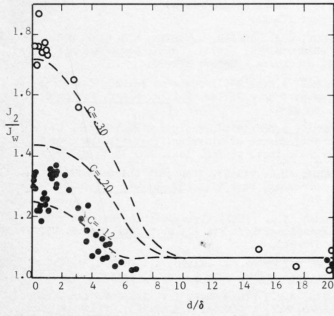
Fig. 4 Variation of $J_2/J_w$ with $d/\delta$ , S.G. 2.65
Experimental $d=\mathrm{.13},\mathrm{.175},\mathrm{.48},1.20$ mm $•C=12\%$
$\circ C=30\%$

4.3 Relation to $\varphi$ - $\Psi$ plots

The change in slope and displacement of data for different pipe sizes evident in Figure 3 at high values of $\Psi$ can now be explained. For this fine 0.13 mm sand the $d/\delta$ ratio is around 3 to 7 which means that the viscosity effects in the wall region are of importance. For the same value of $\Psi$ these effects will be more significant in the smaller pipe diameters giving higher $\varphi$ values. As $\Psi$ continues to be increased eventually in all pipe sizes so that the data for different pipe sizes should converge at very high values of $\Psi$ , a trend which is suggested by the data.

For the coarse 1.2 mm sand of Fig. 2 $d/\delta$ is around 50 and for a concentration of 12% equation 6 gives $J_2/J_w=1.07$ at high velocities, i.e. $\varphi =0.58$ and the result is the same for all pipe diameters so there is no data separation for different pipe sizes, even at high values of $\Psi$ .

5 FLOW IN LOW VELOCITY REGION

Although the displacement of the data points for different pipe sizes evident in Figure 3 has been explained in the region of high $\Psi$ values the displacement at low $\Psi$ values is as yet unexplained. To study this region it is helpful to return to the Durand parameter $\Psi$ which has been seen to successfully correlate the data for coarse sands. It was observed by Durand (1953) that the critical velocity for these suspensions was given by

$$V_c=F_1\sqrt{2gD(S-1)}(7)$$

where $F_1$ is a weak function of concentration but is close to 1.3. Examination of equation 3 will reveal that the variable $\Psi$ does in fact contain $V_c$ and so in equation 4 $\Psi$ could be replaced by the more general $\xi$ given by

$$\xi =3.4\sqrt{C_d{\left(\frac{V}{V_c}\right)}^2}(8)$$

The use of $V/V_c$ has been suggested by Yufin et al (1975).

For coarse particles $V_c$ is given by equation 7 and $\xi =\Psi$ . For fine particles smaller than the viscous sub-layer (i.e. ) D.G. Thomas (1962) has proposed the following equation

$$\frac{W}{V_c^{*}}=0.010{\left(\frac{d{v}_{*}^{*}·\theta }{v_w}\right)}^{2.71}(9)$$

This equation indicates that $V_c$ is approximately proportional to $D_c^{0.1}$ compared with the $D_c^{0.5}$ of equation (7) and this has been experimentally observed (Shriek et al 1973, A.D. Thomas 1975). For particles midway between the fine and coarse extremes such as the 0.13 mm sand of Fig 3 the critical velocity could be expected to vary approximately as $D_c^m$ where $m$ might lie somewhere between 0.1 and 0.5. The actual critical deposit velocities for this sand in the 18.9, 53.8 and 105 mm pipes at $C=12\%$ were 0.80, 1.15, and 1.45 m/s respectively which indicates that $V_c\propto D_c^{0.35}$ because $V_c\approx V_d$ for this sand.

With $V_c$ depending on $D$ in this manner examination of Fig 3 shows that the displacement of the data points at low $\Psi$ values could be eliminated if $\xi$ were used instead of $\Psi$ . Of course the data points for different pipe sizes in this Figure are still displaced at high values but this can be explained and allowed for as discussed in Section 4.

6 COMBINED MODEL FOR HIGH AND LOW VELOCITY REGIONS

To obtain a smooth continuous equation describing the pressure gradient for all velocity values above $V_c$ it is convenient to assume an additive form as

where ${\varphi }_1$ and ${\varphi }_2$ are increasingly important at the low and high velocity regions respectively. Following the discussion in Section 5 a suitable equation for ${\varphi }_1$ is

$${\varphi }_1=80{\xi }^{-1.25}(12)$$

while ${\varphi }_2$ can be obtained by the method of Section 4. Note that both ${\varphi }_1$ and ${\varphi }_2$ are dependent on the ratio $d/\delta$ , the first indirectly through the dependence of $V$ on $d/\delta$ , and the second directly as given by the variance of $J_w/J_w$ with $d/\delta$ in Figure 4. A method of calculating $V^w$ for all $d/\delta$ values is not yet available, however Equations 7 and 9 provide upper and lower limits while the results for the 0.13 mm sand provide data intermediate between these extremes.

Using the observed critical velocity to calculate $\xi$ values of $\varphi$ has been calculated for the 0.13 mm sand in the 18.9, 53.8 and 105 mm pipe sizes, and the results are shown in Figure 5. Although exact agreement is not obtained the general trends of the predicted curves agree with the observed behaviour - namely data from all three pipe sizes converging at the low and high $\xi$ regions but being displaced at intermediate values of $\xi$ . The maximum equivalent error in pressure gradient prediction is 11%.

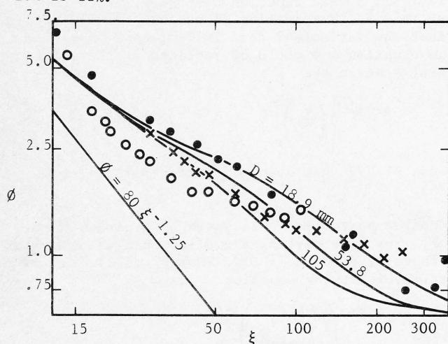
Fig. 5 Variation of $\varphi$ with $\xi$ , $C=12\%$ , 0.13 mm sand • $D=18.9$ mm, $X=53.8$ mm, $O=105$ mm

7 DEPOSIT VELOCITY

The pressure gradient prediction method presented here involves an estimate of $V_c$ . Obviously also of great practical interest is $V_c$ . For fine particles $V\approx V_c$ but for coarse particles in small pipes $V$ can be considerably less than $V_c$ . When a single layer of particles deposits in the pipe the flow area is reduced. The deposit will only remain if the mean velocity above the bed is less than $V_c$ for a pipe of diameter $D$ - $d$ . Further consideration will show that

$$V_d/V_c\approx {\left\{\frac{(D-d)/D}{d}\right\}}^{2/m}(13)$$

where $m$ varies from 0.5 for coarse particles to 0.1 for fine particles.

8 CONCLUSIONS

A careful study of the Durand equation has enabled its main inadequacies to be isolated and studied. The result is a simple but rationally based prediction

which can explain most of the scatter evident on previous $\varphi$ - $\Psi$ plots. The pressure gradient for any size particle in any pipe size can be obtained by applying equation 11. In this equation ${\varphi }_1$ is calculated using equations 12 and 8 along with an estimate for $V_c$ . ${\varphi }_2$ is calculated using equation 5 or 6 along with Figure 4.

9 ACKNOWLEDGEMENT

The author wishes to thank M.D. Research Co. Pty. Ltd. for permission to publish this paper.

10 REFERENCES

BABCOCK, H.A. (1968). Heterogeneous flow of Heterogeneous solids. Int. Symposium on Solid Liquid Flow in pipes , Univ. of Penn. Phil. U.S.A.

DAILY, W.D. and ROBERTS, P.R. (1969). Rigid particle suspensions in turbulent shear flow. Tappi , Vol. 49, No. 3, pp 115 - 125.

DURAND, R. (1953). Basic relationships of the trans portation of solids in pipes. Proc. Minn. Int. Hydr. Conv. , Int. Assoc. for Hydr. Res. pp 89-103.

HAYDEN, J.W. & STELSUN, T.E. (1968). Hydraulic conveyance of solids in pipes. Int. Symposium on Solid Liquid flow in Pipes , Univ. of Penn. Phil.

HINZE, J.O. (1959) Turbulence , McGraw-Hill, New York.

MAUDE, A.D. & WHITMORE, R.L. (1958). The turbulent flow of suspensions in tubes. Trans Inst Chem. Engrs. Vol 36, pp 296-304.

MURPHY G. YOUNG, D.F. & BURIAN, R.J. (1955). Progress report on friction loss of slurries in straight tubes. U.S.A.E.C., Report ISC-474 (79p)

NEWITT, D.M. RICHARDSON, J.F. ABBOTT, M. & TURTLE, R.B. (1955). Hydraulic conveying of solids in horizontal pipes. Trans. Instn Chem. Engrs. Vol. 33 pp 93 - 110.

NEWITT, D.M. RICHARDSON, J.F. & GLIDDON, G.J. (1961) Hydraulic conveying of solids in vertical pipes. Trans. Instn Chem. Engrs. Vol 39, pp 93-100.

SCHRIEK, W. SMITH, L.G. HAAS, D.B. & HUSBAND, W.H.W. (1973). Saskatchewan Research Council of Canada, Report E73-21.

SHOOK, C.A. SCHRIEK, W. SMITH, L.G. HAAS, D.B. & HUSBAND, W.H.W. (1973). Saskatchewan Research Council of Canada. Report E73-20.

THOMAS, A.D. (1976). Scale-up methods for pipeline transport of slurries. Int. J. Miner. Process. Vol. 3, pp 51-69.

THOMAS, A.D. (1975). Factors affecting the hydraulic performance of slurries. Thermofluids conf. Bris. Dec 3-5, Inst. of Eng. Aust. No. 75/9, pp 96-100.

THOMAS, D.G. (1965). Fluid characteristics of suspensions. Part VIII. J. Colloid Sci. , Vol. 20, pp 267.

THOMAS, D.G. (1962). Transport characteristics of suspensions: Part VI. A.I.Ch.E. Jnl , Vol 8, No. 3 pp 373-378.

TODA, M., KONNO, H., SAITO, S. & MAEDA, S. (1969) Int. Chem Engnr. Vol. 9, No. 3, pp 553-560.

YUFIN, A.P., FILIMONOVA, I.V. TARASOV, V.K., DANIL' CHENKO, N.V. & BELOVA, N.T. (1975). Fluid Mechanics - Soviet Research, Vol 4, No. 2 pp 5-8.

ZANDI, I. & GOVATOS, G. (1967). Heterogeneous flow of solids in pipelines. A.S.C.E. H73, pp 145-157.