The role of laminar-turbulent transition in determining critical deposit velocity and operating pressure gradient

Page 1

Hydrotransport 6 PAPER A2

SIXTH INTERNATIONAL CONFERENCE ON THE

HYDRAULIC TRANSPORT OF SOLIDS IN PIPES

SEPTEMBER 26th-28th, 1979

THE ROLE OF LAMINAR/TURBULENT TRANSITION IN DETERMINING

THE CRITICAL DEPOSIT VELOCITY AND THE OPERATING

PRESSURE GRADIENT FOR LONG

DISTANCE SLURRY PIPELINES

A.D. Thomas M.D. Research Company Pty. Ltd., Australia.

Summary

Industrial slurries suitable for pumping over long distances invariably include a proportion of fines which form a viscous "carrier" supporting the larger particles. Viscous effects therefore exert considerable influence on both the critical deposit velocity and the pressure gradient. Because of this it is often assumed that for such slurries the critical deposit velocity coincides with the transition velocity. Here this matter is considered in detail and it is concluded that although the two velocities often do coincide such is not always the case, especially in larger pipe sizes where the critical deposit velocity may be significantly greater than the transition velocity.

Experimental data obtained mostly in a 105mm pipe loop with both high viscosity

Newtonian fluids and clay/water suspensions forming the "carriers" is used to illustrate the controlling phenomena. The reason why the critical deposit velocity and the

transition velocity often do coincide is shown to result from the high pressure gradients

required to prevent deposition under laminar flow conditions. Based on these findings the variation of deposit velocity (and hence the operating pressure gradient) in large pipe sizes is outlined.

Held at University of Kent, Canterbury, U.K. Conference Organised by BHRA Fluid Engineering, Cranfield, Bedford, England. © Copyright BHRA Fluid Engineering

13

Page 2

NOMENCLATURE

Fraction of pipe area above sliding bed Concentration by volume of solids Concentration at maximum packing density (usually taken as 0.6) D Pipe diameter Fanning friction factor for flow of fluid or vehicle Gravitational constant

J Slurry pressure gradient Ja Slurry pressure gradient at incipient deposition Re Reynolds number (= VD p/ n)

S Relative solids density in carrier fluid or vehicle Mean flow velocity in pipe Mean velocity at incipient deposition Vt Velocity of transition between laminar and turbulent flow V

d * Friction velocity at incipient deposition (= VaVF/2)

n l Dynamic viscosity of Newtonian fluid

e Effective viscosity of non-Newtonian vehicle npl Plastic viscosity of Bingham plastic vehicle H s Co-efficient of sliding friction between sliding bed & pipe (usually taken as 0.4)

Density of fluid or vehicle Yield stress of Bingham plastic Function appearing in equation 5 and given in Ref. 4. For C=.12, Ø = 0.26

The thickness of the viscous sublayer which has not been given a

specific symbol is given by 5n/pV*

14

Page 3

1. INTRODUCTION

Long distance pipelines transporting slurried minerals are a reality, with many examples operating successfully throughout the world. In spite of this the hydraulic design of such pipelines is still clouded in some mystery, as has been indicated by Carleton & Cheng (Ref. 1), with the design often being described as more of an art than a science. Particular mystery surrounds the role of the laminar/turbulent transition in determining the critical deposit velocity (the velocity at which a stationary deposit first appears) and hence the operating pressure gradient. It is often assumed (e.g. Hanks, Ref. 2) for typical pseudo-homogeneous slurries pumped in long distance applications that the critical deposit velocity coincides with the velocity of transition between laminar and turbulent flow. In this present paper the relationship between these two velocities is studied, firstly for sands in high viscosity Newtonian fluids, and then for more typical non-Newtonian based slurries. This paper in effect fills in the gap between the two recent papers by the author (Thomas, Refs. 3 & 4). The first of these considered the critical deposit velocity under conditions of pure turbulent flow while the second considered deposition under conditions of pure laminar flow.

2. EXPERIMENTAL EQUIPMENT

The pipe 1oops used have been described elsewhere (Thomas, Ref. 5). They were conventional types of various diameters ranging from 9.41 to 105 mm. Flow rates were measured by diverting the flow into a weigh tank except in the case of high viscosity Newtonian fluids (sugar/water solutions) where a venturi was used. Concentrations were measured by weighing a known volume of sample. Pressure gradients were measured over horizontal lengths of pipe using a transducer. Critical deposit velocities were determined by observation through transparent viewing sections. This method could also be used to determine the laminar/turbulent transition velocity since transition was clearly evident by the presence of bursts. A more clearly defined transition velocity was obtained by the intersection of the laminar and turbulent pressure gradient plots. Newtonian fluid viscosities were measured using a Brookfield was obtained in a tube viscometer. rotational viscometer whilst the rheological behaviour for non-Newtonian suspensions

3. TYPICAL BEHAVIOUR - NEWTONIAN FLUIDS

The area of interest of the present paper is best illustrated by some typical pipe loop results. are for nominal 0.15 mm (90% between 0.095 and 0.30 mm) silica sand in Newtonian fluids (sugar/water solutions) of various viscosities. Figure 1 shows the result obtained in the 105 mm pipe at four different viscosities, 0.80, 5, 60 and 95 centipoise (cp), the respective fluid densities being 996, 1160, 1300 and 1315 kg m -3 The solids concentration was 12% by volume. Note that the results for the two highest viscosities have been presented previously (Ref. 4) whilst the deposit velocities for the two lowest viscosities were used in Ref. 3. lowest viscosity the behaviour is typical of heterogeneous slurries. would not be considered for long distance transportation because, as has been explained by Thomas (Ref. 6), the required pressure gradient is uneconomic in large pipe sizes. At a viscosity of 5 cp typical pseudo-homogeneous behaviour is apparent as evidenced by the parallelling of the slurry data points to the fluid line. From a pressure that deposition occurs which is well above the transition regime. gradient viewpoint such a slurry would be at a Reynolds number, based on fluid properties, of 2x10dote suitable for long distance pumping. Deposition is therefore occurring in pure turbulent flow and the deposition criterion presented by Thomas (Ref. 3) is applicable. When the fluid viscosity is increased to 60 cp deposition is now seen to occur at a Reynolds number of 2900 which is in the middle of the transition regime commonly assumed to lie between Reynolds numbers of 2000 and 4000. For this slurry the assumption that deposition coincides with laminar/turbulent transition is therefore number of 1300 under conditions of pure laminar flow. Finally, at the highest viscosity of 95 cp, deposition occurs at a Reynolds For predicting the critical deposit velocity in this case the work of Thomas (Ref. 4) is relevant.

15

Page 4

of interest is further illustrated by Fig. 2. Shown on this Figure are data for three different pipe sizes for the one sand (median size 0.13 mm with 90% between.095 and.155 mm) at the one concentration (12%) and fluid viscosity of 5 cp. Of this data the 9.41 mm pipe results have previously been presented (Ref. 4) whilst the deposit velocity result for the 105 mm pipe was used in Ref. 3. It can be seen that deposition occurred in the laminar regime in the 9.41 mm pipe, in regime in the 18.9 mm pipe, and well into the turbulent regime in the 105mm pipe. These results are for a particular slurry in different pipe sizes. They graphically illustrate why it cannot be assumed that, for a particular slurry, the deposit velocity will coincide with the transition velocity for all pipe sizes.

4. PREDICTING THE DEPOSIT VELOCITY - NEWTONIAN FLUIDS

4.1 Turbulent FLow

As noted previously only pseudo-homogeneous slurries need be considered for

distance applications. slurries the critical deposit velocity according to Thomas (Ref. 3) is given by

v = 1.1 [8n (S-1)/ o) (1)

Equation 1 was obtained by applying Wilson's (Ref. 7) sliding bed theory to a sliding bed of height equal to the viscous sub-layer. (see nomenclature) Employing the definition of friction velocity and the Blasius type approximation for the friction factor suggested by Knudsen & Katz (Ref. 8), namely

£ = 0.046 Re-0.2 (2)

equation 1 can be approximated by

Va = 9.087 (5-1)/ 10.31 (DP/n) 0.11 (3)

S.I. units being used. Also of great practical importance is the pressure gradient at deposition, Ja

which as a first approximation can be assumed equal to the fluid only pressure

gradient multiplied by the ratio of the slurry density to fluid density. The result can be shown to be;

Ja = 4.4 [1 + C(5-1)] [8 n(S-1)/0|30/D (4)

Alternatively, if greater accuracy is required, the effect of the solids on the slurry viscosity can be taken into account as considered by Vocadlo (Ref. 9). 4.2 Laminar Flow By a similar application of Wilson's sliding bed theory Thomas (Ref. 4) showed that the slurry pressure gradient at deposition under laminar flow is given by

Ja = 208 4s C,(5-1) 8 (5)

As a first approximation the in-situ concentration can be assumed equal to the delivered concentration. enable full settling of the particles, equation 5 can be used to calculate Ja• the pipe loop is of insufficient length to obtain full settling of all the particles then the pressure gradient at deposition will be less than given by equation 5 because the height of the sliding bed will be less with some of the particles still in suspension (see Thomas, Ref. 4). Note that equation 5 is independent of pipe size. It will be seen later that the physical mechanisms of deposition can best be

understood in terms of Ja but if it is required, the deposit velocity can be obtained

16

Page 5

by equating Ja to the pressure gradient due to laminar flow in the reduced pipe area above the bed. A full analysis is not warranted here but as a first approximation V d will depend on the following proportionality.

(6)

Vote that for a given solids concentration (a and D, constant) n needs to be increased in proportion to D' to maintain the same deposit velocity in larger pipes.

4.3 Transition Regime

of 3000. The middle of the transition regime can be assumed to occur at a Reynolds number Thus for these situations where deposition coincides with transition Va equals Vt where Vt is given by

Vt = 3000 n (7)

Do

the slurry pressure gradient equals the fluid only pressure gradient times the ratio of slurry density to fluid density. can be calculated accordingly by assuming that, as in the turbulent case, that 4.4 Example (One Slurry, various pipe sizes) Using the above equations J The result is shown in Fig. 3 together with the experimental data. has been calculated for the conditions relating to seen that there is only a small range of pipe sizes, from 13 to 21mm, in the transition region. For pipe sizes above 21 mm the deposition

occurs under conditions of pure turbulent flow and the pressure gradient at deposition (and the velocity) are considerably higher than the transition value. An insight into the physical reasons for the co-incidence of deposition and transition can be obtained by tracing the behaviour as the pipe size is progressively decreased. In large pipe sizes deposition occurs under purely turbulent flow but at a pipe size of 21 mm the transition velocity has risen up to first coincide with deposition. Further reduction in pipe size still sees deposition coinciding with transition because the pressure gradient is insufficient to maintain pure laminar flow without deposition. pipe size is reduced to below 13mm that the pressure gradient is sufficient to maintain laminar flow without deposition. For a higher viscosity fluid the required pressure gradient for laminar flow operation can be reached in a larger pipe. For example for a 50 cp fluid deposition will coincide with transition in pipe sizes from 60 to 100 mm as indicated on Fig. 3. Thus for Newtonian fluids the two velocities will coincide over a pipe size range of approximately 2 to 1 with the actual pipe sizes depending on the viscosity. 4.5 Example (One pipe size, various viscosities) Further insight into the physical mechanisms involved is provided by Fig. 4 which shows results for 12% concentration of 0.82 mm silica sand (90% between 0.60 and 1.05 mm) in the 105 mm pipeloop at various fluid viscosities. Note that the results for 270 cp have previously been presented (Ref. 4). The fluid density was

1300 kg m-3 so equation 5 indicates that for laminar conditions, Ja = 1650 Pa m-1

Thus, the theory indicates that to obtain laminar flow without deposition a pressure gradient at least as great as this is necessary. At the lowest viscosity of 56 cp deposition occurs at a Reynolds number of 3450, i.e. under conditions of almost pure turbulent flow and the pressure gradient is low at 700 Pa mI In this case the height of the sliding bed will be not much higher than the viscous sub-layer thickness. At a viscosity of 82 cp deposition occurs just below the transition regime at Re = 1800 Note that Ja has risen to 900 Pa m-l due to a greater bed height because of less turbulent support of particles. However the viscosity is not sufficiently high to sustain laminar flow without deposition, which theoretically at least, requires a pressure gradient of 1650 Pa m At a viscosity of 119 cp J has risen to 1150 Pa m and although the Reynolds number at deposition is less than 2000 pure laminar flow was not yet obtained as evidenced by visual observation of transition bursts.

17

Page 6

viscosity of 175 cp pure laminar flow was sustained. Deposition occurred at a pressure gradient of 1200 Pa m-l, somewhat below the theoretical value of 1650. At the highest viscosity of 270 cp laminar flow is obtained over a considerable range of

velocities. different from the theoretical value of 1650 Pa m'l. Deposition occurred at a pressure gradient of 1450 Pa m-l, not too

The physical mechanisms involved as the viscosity is increased can now be At low viscosities deposition occurs under turbulent flow with the height of the sliding bed being as great as the viscous sub-layer thickness. tly the required pressure gradient As the viscosity is increased the transition regime rises up to the velocities of interest. When this happens turbulent support of particles is reduced and the bed height increases, requiring higher pressure gradients. Eventually at still higher viscosities pure laminar flow is obtained. the bed height is determined by the in-situ solids concentration and is much higher than that which was present under turbulent flow. This requires a high pressure gradient as per equation 5 and this can only be obtained if the viscosity is raised sufficiently high. For a particular pipe size it is only in the range, where the viscosity is high enough to prevent deposition occurring in the turbulent regime, but not high enough to sustain pure laminar flow, that the deposit velocity coincides with the transition velocity.

5. BEHAVIOUR OF REAL SLURRIES

With practical pseudo-homogeneous slurries the coarser particles are suspended,

not in a viscous Newtonian fluid, but in a "vehicle" or "carrier" pseudo-fluid which is a suspension of the very fine particles of size maybe less than 10 to 20 microns. Because of the requirements for a long distance type slurry to be stable on shutdown it is necessary that these "fines" be flocculated (see Thomas, Ref. 6) giving the vehicle non-Newtonian properties including a yield stress. They can loosely be termed Bingham plastics. Qualitatively such slurries follow the same behavioural pattern as the Newtonian fluid based ones. For example Fig. 5 shows results obtained in the 105 mm pipe loop with 0.15 mm silica sand (90% between 0.1 and 0.26 mm) suspended in flocculated clay suspensions of various concentrations. The results for the two highest concentrations have previously been published (Ref. 5). The concentration of the sand in the clay suspension varies from 16.8% by volume at zero clay concentratat a clay concentration of 6.2%. The dry solids density of the clay

2370 kg m-3, The full lines indicate the behaviour of the clay suspensions alone.

The behaviour is qualitatively similar to that in Fig. 4, i.e. increasing clay concentration is analogous to increasing viscosity. clay concentration deposition occurs under conditions of pure turbulent flow. An increase in clay concentration initially causes a slight increase in the deposition velocity. in keeping with the positive influence of viscosity in equation 3. At higher clay concentrations the deposition velocity coincides with the transition velocity. clay concentration continues to be increased eventually the consistency is sufficient to permit laminar flow without deposition. Tests by the author have also confirmed that the behaviour of a particular real slurry in various pipe sizes is qualitatively similar to that observed with

Newtonian based slurries (illustrated by Fig. 2). Unfortunately this data is

proprietary information and cannot be presented,

6. PREDICTING THE DEPOSIT VELOCITY - REAL SLURRIES

Although the equations developed for Newtonian based slurries and presented in Section 4 are applicable in principle to non-Newtonian based slurries, their use is subject to some uncertainties. 6.1 Turbulent Flow In applying equations 1 or 3 to non-Newtonian vehicles the problem lies in selecting a suitable value of viscosity. D.G. Thomas (Ref. 10) has argued that the

18

Page 7

relevant viscosity under turbulent flow conditions is the effective viscosity at infinite shear rate, which for a Bingham plastic is equal to the plastic viscosity, P=Bportioney tone Squation 1 was derlved by assuming lowever he found this there was a slight thickening of the viscous sub-layer where n is the viscosity of the suspending medium (water). get on in eat be ented at hide does not super is to one on., the height of the sliding bed equalled the thick- The author has not considered this for a Bingham plastic should ben For example consider the 3.6% clay concentration result of Fig. 5 for which i.e. as From equation 3 this results in an equivalent viscosity of.01 Nsm-2 far as deposition is concerned this clay suspension is behaving as a Newtonian fluid = 3 cp, less than one of viscosity 10 cp. n. Pthird of the equivalent viscosity. Better for this suspension was 2.6 cp so that pl agreèment is obtained wall if the effective viscosity, Me, obtained from the laminar flow curve, for the relevant stress is used, e.g. in the above casene =7.3 cp. The use of ne in equations 1 or 3 needs to be tested over a much larger range of data before it can be recommended for general use. in practice, even without this uncertainty, equations 1 & 3 would need to be used with caution because ofthe problem in defining the vehicle portion of a slurry. In the example above relating to Fig. 5 there is no problem in defining the vehicle portion - it is quite clearly the clay suspension. However most slurries will not have such a clearly defined demarcation. They will generally have a continuous size distribution making separation of the vehicle portion difficult. This obstacle can be overcome quite simply however by using equations 1 & 3 merely as scale-up relations. Suppose tests are performed on a particular slurry in a small diameter pipe and it is found that the slurry behaves pseudo-homogeneously and deposits out at a certain velocity. Provided fully turbulent flow was present, and this could be checked by tests in a o no. 1 lightly from equation 3. by Schriek et al (Ref. 11) in pipe sizes from 50 to 300 mm amply demonstrate this fact as can be seen in Fig. 6. Just as with Newtonian fluids the pressure gradient at deposition can be obtained by multiplying the vehicle only pressure gradient by the ratio of slurry density to vehicle density. Alternatively, and more accurately, the pressure gradient can be obtained by scaling up from the small pipe loop results. i.e. by multiplying the vehicle only pressure gradient by the same factor as indicated by the results in the smaller pipes. A third alternative is to scale up the actual slurry results using the method of Bowen (Ref. 12). 6.2 Laminar Flow No reliable deposition criterion exists at present for the laminar flow of slurries composed of coarse particles in a flocculated fine particle vehicle, the so called stabilized slurry. Use of equation 5 often results in severe overprediction. Thomas (Ref, 4) recently considered this and has suggested that the discrepancy is a less compact sliding bed. The particles are apparently kept separated by the structure of the vehicle thereby reducing particle/particle interaction and reducing the pressure gradient. Although quantitative prediction is not possible it can safely be stated that the pressure gradient required to prevent deposition under laminar flow will always be greater than that required under turbulent flow for the same coarse particles. 6.3 Transition Regime as with the Newtonian fluid based slurry the deposit velocity will coincide with the transition-velocity for some slurry and pipe size situations. these cases once again the pressure gradient at deposition can be estimated by multiplying the vehicle only pressure gradient by the ratio of slurry density to vehicle density or by scale up from the results of small pipe tests.

19

Page 8

7. DESIGN EXAMPLE

Because of the uncertainties associated with the prediction of deposition under laminar and turbulent conditions for real (flocculated) slurries the design must proceed on the basis of scale up of small pipe loop results. The procedure to be followed can best be understood by working through a typical design example. Unfortunately limited data obtained in only two pipe sizes is available. To help in illustrating the procedures fictitious data for two other pipe sizes will also be presented. Fig. 7 shows results obtained in the two pipe sizes, 18.9 and 105 mm, with a 32% concentration of loam slurry (mixture of sand and clay, solids density 2540 kg m-3). Also shown are fictitious data showing likely behaviour in 40 and 200mm pipes. 7.1 Scaling-up of Laminar Flow Data

velocitrethe 11o9 as pope marinandicating pseudo-homogen us, indicating pseudo-homogeneous behaviour. possible down to This data,

plotted as wall shear stress (DJ/4) versus apparent shear rate (8V/D), represents the flow curve for this slurry from which the theoretical laminar behaviour in any pipe size can be calculated. The resulting laminar flow curves are shown as dashed lines on Fig. 7 although it must be remembered that as the pipe size is increased deposition may occur before such laminar flow can be realized as is seen to occur with the 105 mm and 200 mm pipes. The fictitious data for the 40 mm pipe indicates laminar flow was obtained but this data would not be suitable for determining the flow curve because of the distortion due to settling effects. 7.2 Predicting the Transition Velocity

= 10 Pa and Mp1 = 9 x 10-3 NSm 2 was most appropriate. A linear plot of the above flow curve indicated that the Bingham model with a

Govier & Aziz (Ref. 13)

have considered a number of methods of predicting the transition velocity for Bingham plastics. Perhaps the most commonly used is the one obtained by analogy with Newtonian fluids, namely that transition occurs when

D V t = 2100 (8) 1 + T D

For this slurry in a 18.9 mm pipe this equation gives V.. = 1.9 ms-1, in close agreement with the observed 2 ms-l An alternative prediction method has been

Booped bys aaks Rised to predict in transit on velocity in aly sine pope but ten, also in good agreement.

two methods result in predictions increasingly different as the pipe size is increased. Hanks' method indicates a steady decrease in Vt as D is increased whereas equation 8 gives Vt asymptotically approaching a constant value of 1.60 ms-1 in large pipe sizes. It is beyond the scope of the present paper to resolve this discrepancy. Hanks' value of Vt will be taken as a lower limit and the value obtained using equation 8 will be taken as the upper limit. The resulting transition band is in Fig. 7. 7.3 Scaling-up of the Deposit Velocity From Fig. 7 it can be seen that deposition occurred within the transition band mm pipe, i.e. that deposition coincided approximately with transition. However, as has been shown in previous sections, this does not mean that deposition will coincide with transition in larger pipe sizes. This is illustrated by the fictitious data for the 200 mm pipe which shows deposition occurring well into the turbulent regime. With data such as on Fig. 7 available the prediction of the deposit velocity for this slurry in large pipe sizes proceeds by scaling up the result for fully

20

Page 9

turbulent deposition in the 200 mm pipe using equation 3, i.e.

VIa DO.11 (9)

as is shown in Fig. 8. The pressure gradient at deposition can be obtained simply by multiplying the calculated pressure gradient for water alone at velocity V ratio of the slurry density to the water density or more accurately by scaling up the by the results in the smaller pipes. This example has served to illustrate the method which must be followed to predict the deposit velocity. For the particular slurry considered it is evident that deposition only co-incides with transition for pipe sizes approximately between 100 and 200 mm, i.e. a similar 2 to 1 pipe size range as occurred with Newtonian fluids (Section 4.4). For pipe sizes greater than 200 mm deposition occurred above the transition velocity. Note that to predict the deposit velocity in these large pipes it is necessary that tests be carried out in a pipe of size sufficiently large that deposition occurs under pure turbulent flow. For this particular slurry this required a pipe size of 200mm. However, this slurry would not be suitable for long distance pumping because the deposit velocity in large pipe sizes is above the normal

economic pumping velocity of about 1,75 ms"1 monomic velocity restriction means that deposit belodies sed nd Tmas Ref. 6)

For such slurries tests in pipes no larger than about 100 mm are sufficient to obtain deposition under fully turbulent flow. For example the iron ore concentrate tested by Schriek et al (Ref, 11) would be a suitable slurry for long distance app 6, long as the deposit elos yury aroned toughly as olevaty en, Fig. 6, that deposition even for a pipe size as small as 50 mm. For this slurry it is obvious, indicating turbulent that tests in the 50 and 100 mm pipe would be sufficient to confirm that deposition was occurring under turbulent flow.

The common assumption that for long distance type slurries the critical deposit velocity coincides with the laminar/turbulent transition velocity has been shown to be in general incorrect although for any particular slurry there will be a limited range of pipe sizes (generally about 2 to 1 ratio) for which the two velocities will As the pipe size is reduced within this range deposition will continue to be determined by transition until the pressure gradient rises sufficiently to permit laminar flow without deposition. For pipe sizes below this range deposition will occur under laminar flow conditions whilst for pipe sizes above this range deposition will occur under conditions of pure turbulent flow. To predict the deposit velocity in large pipe sizes it is necessary to perform pipe loop tests in a pipe of size sufficiently large that deposition occurs under conditions of pure turbulent flow. For typical long distance type slurries this necessitates tests in pipes up to about 100 mm diameter.

ACKNOWLEDGEMENT'S

The author thanks M.D. Research Company Pty Limited for permission to publish this paper.

10. REFERENCES

1. CARLETON, A.J. and CHENG, D. C-H, "Pipeline design for industrial slurries" Chemical Engineering, April 25, PP 95-100 (1977). 2. HANKS, Res, " Proc. 3rd Int. Tech. Conf. on Slurry Transportation, Las Vegas, Organized by Slurry Transport Association, Washington D.C. "The 'influence of slurry rheology on turbulent pipeline hydraulics,' (March 29th - 31st, 197'). THOMAS, A.D., "Predicting the deposit velocity for horizontal turbulent pipe flow of slurries," submitted to Int. Jnl. of Multiphase Flow, July, 1978.

21

Page 10

4. THOMAS, A.D., "Pipelining of coarse coal as a stabilized slurry - another viewpoint, presented at 4th Int. Tech. Conf, on Slurry Transportation, Las Vegas. Organized by Slurry Transport Association, Washington, D.C. (March 28th-30th, 1979). 5. THOMAS, A.D., "Coarse particles in a heavy medium - turbulent pressure drop reduction and deposition under laminar flow," Proc. 5th Int. Conf. on the Hydraulic Transport of Solids in Pipes, Hannover. Paper D5, Organized by Brit, Hydromech. Res. Assoc., Cranfield. (May 8th-l1th, 1978). 6. THOMAS, A.D., "A rational design philosophy for long distance slurry pipelines" Chemical Engineering in Australia, PP 22-33. (1977). 7. WILSON, K.C., "Co-ordinates for the limit of deposition in pipeline flow," Proc. 3rd Int. Conf. on the Hydraulic Transport of Solids in Pipes, Golden, Colorado, Paper El. Organized by Brit. Hydromech. Res. Assoc., Cranfield. (May 15th-17th, 1974). 8. KNUDSEN, J.G. and KATZ, D.L., "Fluid dynamics and heat transfer, " McGraw-Hill, New York, 1958. 9. VOCADLO, J.J., "Role of some parameters and effective variables in turbulent slurry flow, " Proc. 4th Int. Conf. on the Hydraulic Transport of Solids in Pipes, Banff, Canada, Paper D4. Organized by Brit. Hydromech. Res. Assoc, Cranfield. (May 18th-21st, 1976). 10. THOMAS, D.G., "Transport characteristics of suspensions: Part IV. Friction loss of concentrated-flocculated suspensions in turbulent flow," A.I. Ch. E. Jnl, 8, 2, PP 266-271 (May, 1962). 11. SCHRIEK, W., SMITH, L.G., HAAS, D. and HUSBAND, W.H.W., "Experimental studies on the hydraulic transport of iron ore, " Report E73-12, Saskatchewan Research Council, Saskatoon, Canada (July, 1973). 12. BOWEN, R.L., "Designing turbulent flow systems, " Chemical Engineering, July 24, pp 143-150 (1961). 13. GOVIER, G.W. and AZIZ, K., "The flow of complex mixtures in pipes," Van Nostrand Reinhold, New York (1972). 14. HANKS, R.W., "The laminar-turbulent transition for fluids with a yield stress." A. I. Ch. E. Jnl, 2, 3, PP 306-309 (May, 1963).

22

Page 11

8 0-92 ms 1 95 cp 60 cp 5 cp 0•8 cp

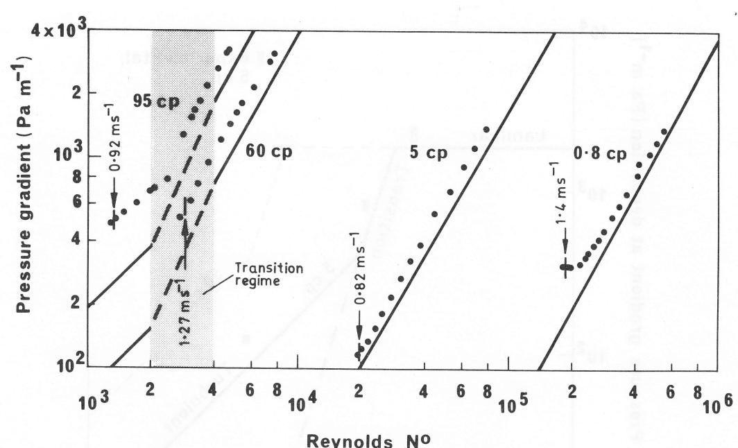
Pressure gradient (Pa m 1) 4x103 Fig. 1. Experimental results for nominal 0. 15 mm sand in fluids of 102 various viscosities in 105 mm diameter pipe. Concentration 12% by 103 2 4 regime Transition 6 8 104 Reynolds No 0-82 ms-1 2 4 6 8105 2 4 6 8106 volume. Full lines indicate laminar and turbulent behaviour for fluid alone. Deposit velocities as indicated.

104 /

gradient ( Pa m-1) 0•2 ms 9.41 mm 18-9 mm

105mm

Pressure 2 Transition regime 0•82 ms'

102 102 2 6 8 103 2 6 8 104 2 6 105

Reynolds N°

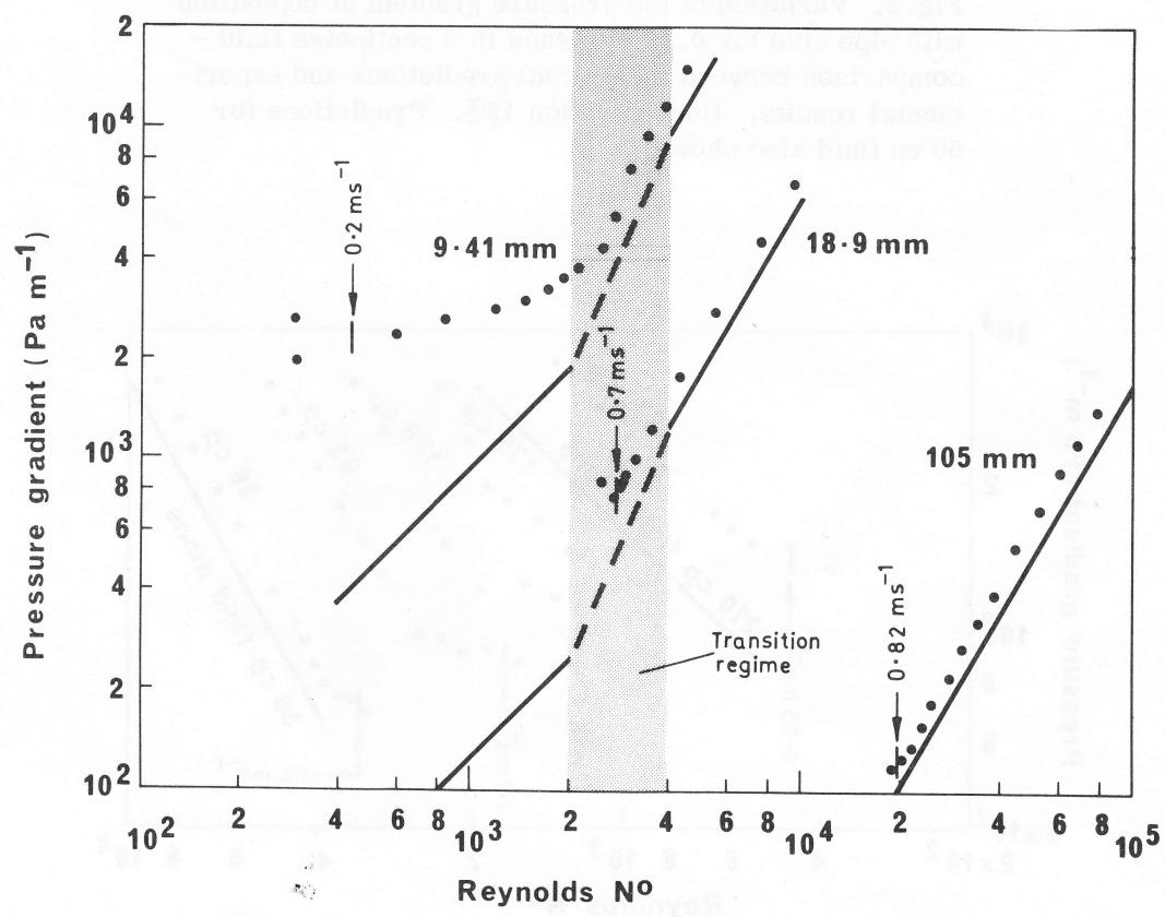
Fig. 2. Experimental results for 0.13 mm sand in three different pipe sizes in a fluid of viscosity 5 centipoise. Concentration 12% by volume. Full lines indicate laminar and turbulent behaviour for fluid alone. Deposit velocities as indicated.

23

Page 12

I Experimental, 5 cp

Laminar

Pressure gradient at deposition (Pa m-') 104 So Turbulent 150

10 1 10 100 1000 Pipe diameter (mm)

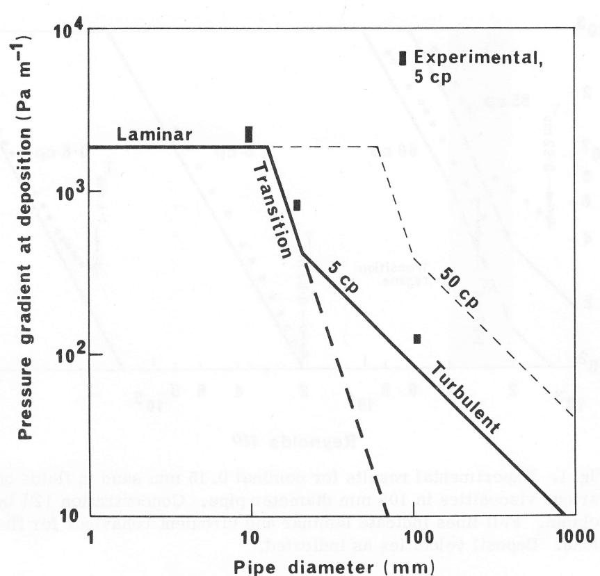
Fig. 3. Variation of the pressure gradient at deposition with pipe size for 0.13 mm sand in 5 centipoise fluid comparison between theoretical predictions and experimental results. Concentration 12%. Predictions for 50 cp fluid also shown.

2 alone 55°

gradient ( Pa m-1, 103 104 fluid: •|° fluid alone

Pressure 0-85 ms l 1.1 ms' 1•1ms-1 1-1 ms 1 - 14 m5' 56

4x102 2x102 4 6 8 103 2 4 8 104

Reynolds N°

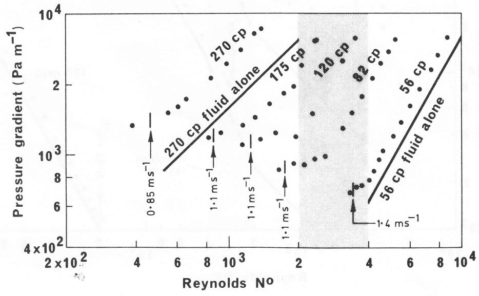
Fig.4. Experimental results for 0.82 mm sand in fluids of various viscosities in 105 mm pipe. Concentration 12%. Shaded area indicates transition regime. Deposit velocities as indicated.

24

Page 13

GRADIENT (Pa ma' PRESSURE a co 6-2% + 0•5 ms-1 5•25% 4-4% 0-7 ms 1 9+1-1m51 =+0-95 ms -1

3.6%

2

10 •1 •2 • 4 • 6 •8 1 2 4 •4 • 6 • 8 1 2 4 6 8 10

VELOCITY ( ms -1,

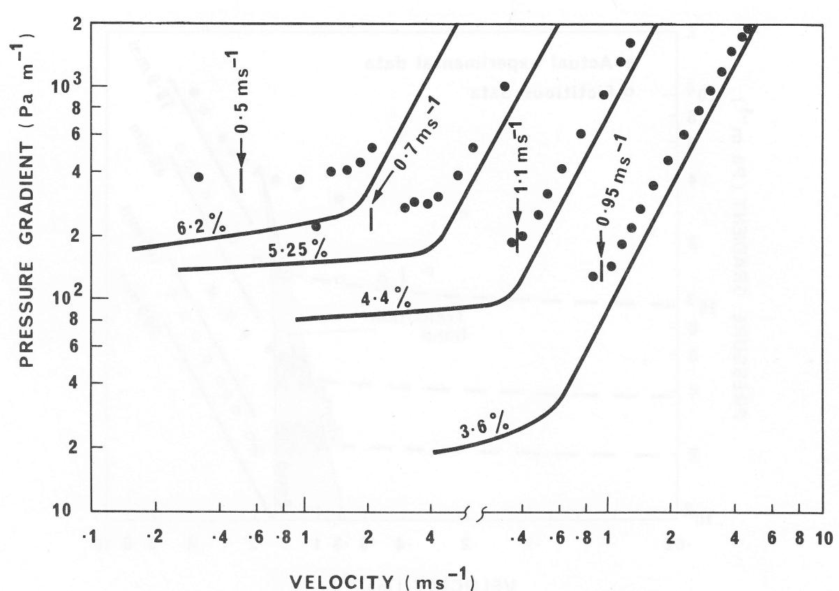
Fig. 5. Experimental results for 0. 15 mm sand in clay suspensions in various concentrations in 105 mm pipe. Nominal sand concentration, 16%. The two scales on the abscissa refer to the 6.2 and 3.6% clay concentrations. Scales for the other two concentrations can be inferred. Deposit velocities as indicated.

1• • 5 Slope 0•11

Deposit velocity (ms), 0-6 • 8 1 2 40 1 1 Pipe diameter (mm) 100 LIlI 200 400

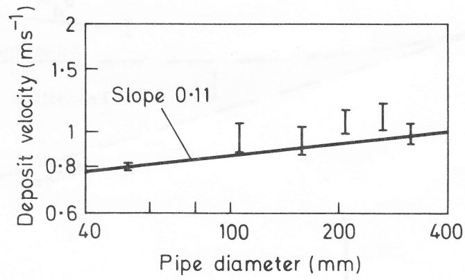
Fig. 6. Variation of deposit velocity with pipe size for iron ore concentrate tested by Schriek et al (Ref. 11). Concentration 30%.

25

Page 14

• 00 40mm

• 105mm

PRESSURE GRADIENT ( Pa m-') 103 104 6 • Actual experimental data • Fictitious data band Transition (Hanks! 1° 18•9 mm 200mm

2

102 •02 • 1 • 2 • 4 • 6 •8 1 2 4 8 10

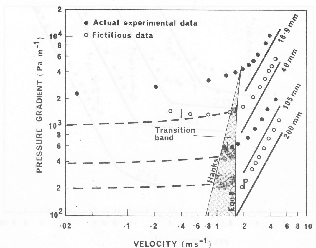
VELOCITY (ms-', Fig. 7. Behaviour of loam slurry in various pipe sizes.

Va<D 0-11

Equation 8

1•0

VELOCITY (m s Transition band Hanks

• 8

•4

•2 10 ~20 40 60 80 100 200 400 600 1000

PIPE DIAMETER (mm)

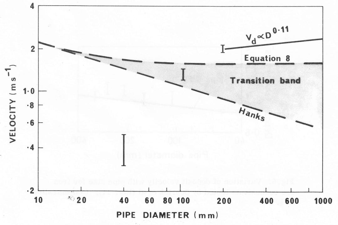
Fig. 8. Deposit velocity scale-up procedure for loam slurry.

26