High density coal ash slurry transport

Page 1

lecture Paper

Power Generation School,

Univ -o WA-

Jan. 1989

HIGH DENSITY COAL ASH SLURRY TRANSPORT

By Allan Thomas Slurry Systems Pty Ltd, PERTH

1. INTRODUCTION

The conventional method of disposing of flyash is to mix it with water to form a low density slurry and then pump it to ponds. Typically the solids concentration is about 30% by weight. This low solids concentration means large quantities of water need to be pumped with consequent large pipe sizes.

An attractive alternative is to pump the flyash at concentration, around 70%. Much less water is required and hence a smaller size pipe can be employed. density slurry advantages disposal site. Because of its high density the slurry is sufficiently thick to sloping deposit which maintains its slope when flow stops. If discharged from a single discharge point, the slurry will form

surface slope of a few percent.

The perimeter of the deposit is determned by

also determines the deposit slope and the

volume of material in the deposit. No perimeter are needed to contain the deposit.

2. FLYASH SLURRY PROPERTIES

1 shows a typical particle size distribution. top size is around 150 microns with the median particle size 15 to 20 microns. Typical solid specific densities

can range between 2200 to 2700 kg/cub. metre.

At low solid concentrations, less than 40 to flyash slurry behaves as a settling slurry ie. if left to stand in a container, the solids will settle to the For pipeline transport, the particles must be supported by the turbulent eddies. The solids increase the effective viscosity of the slurry. This viscosity can be measured in a viscometer. Once the concentration exceeds a certain critical value, typically 40 to 50%, particle interaction becomes significant and the slurry begins to exhibit Newtonian characteristics. shows schematically rheological plots of shear stress versus For a Newtonian fluid the plot passes through the The slope of the line is the viscosity. the critical concentration, the non-Newtonian behaviour can most easily be described by the Binghan plastic

Page 2

model.

T= Ty + 28

Where Ty is the yield stress and n is the plastic viscosity. This yield stress must be exceeded before any shearing can take place. The slope of the line above this stress level is termed the plastic viscosity. At stress levels below the yield value the slurry behaves as an elastic solid. practical effect of this can be observed when pumping such a slurry. If a centrifugal pump connected horizontal pipeline is slowly increased in speed the pressure will slowly rise. However, no flow will take place until the pressure reaches a certain value such that the yield stress

exceeded. This is in contrast with for example water,

where a small flow will occur even for the smallest applied pressure. The presence of a yield stress causes the slurry to become non-settling in nature. The elastic structure can support the coarsest particles thereby preventing settling and any segregation of particle sizes. (1977) gave the following equation required minimum stress required to prevent settling of particles of size d.

Ty = kgd (Pp -P) (1)

Where Pp is the particle density, P is the slurry density and g is the gravitational constant. For isolated coarse particles in an otherwise fine particle slurry, the value of the constant k was Howver, slurries having a continuous size distribution where the coarser particles also contribute to the rheology k was given as 0.46. For a maximum particle size of 150 microns this indicates a required yield stress of between 0.5 and 1 Pascal.

Fig. 3 shows some typical rheology curves for a flyash slurry. Both the yield stress and the plastic viscosity are seen to be strong functions of solids concentration. For this particular slurry a yield stress of 0.5 to 1 is reached at around 60% concentration.

2

Page 3

3. PIPE FLOW BEHAVIOUR AT LOW DENSITIES

3.1 Pseudo-homogeneous Flow

At sufficiently high velocities, the slurry will behave

as a pseudo-homogeneous fluid having near Newtonian properties ie. the turbulent flow friction factor in smooth pipes is determined by one parameter only, the Reynolds number given by Re = VDP//l (2)

The Nikuradse smooth wall equation is

JA=2:5 Ln (Re Inta) (3)

where fN is the Fanning Friction factor given by

AP L (4)

For rough walled pipes, the Colebrook-white equation is generally employed.

- = 4 Log 2k +3:48 - 4 Log (1+9-35- 1(5)

Where k is the pipe roughness. For new steel pipe K =. 05 mm although with slurries the pipe is often smoothed due to slurry abrasion and k can end up closer to.01 mm.

Equation 5 is the basis of the common friction factor charts. It can be used to give an approximate value for the friction factor in the pseudo-homogeneous region although there is an additional complicating issue due to viscous sub-layer effects. During turbulent pipe flow, a thin boundary layer exists adjacent to the pipe where viscous forces predominate. This is termed the viscous sub-layer. Its thickness 8 is given by

3

Page 4

(6)

The thickness of this layer is quite small. For example for water flowing 4m/s in a 100mm pipe equation 6 indicates 8 = 30 microns. For more viscous fluids or slurries 6 is larger. Consider the flow of a low concentration flyash slurry for which the viscosity is similar to that of water. For the above conditions where 8 = 30 microns, only particles significantly smaller than this will be able to

physically "fit" into the sub-layer. Particles larger

than 8 will therefore not be able to contribute to any

viscosity increase within the sub-layer. For the size

distribution Fig. 1 about 40% of the particles are larger than 30 microns. This means that the effective slurry viscosity the viscous sub-layer is less than the full slurry viscosity. This results in the friction factor being less than that calculated using the measured slurry viscosity. As the flow velocity decreases, & increases. This means a greater proportion of the particles are smaller than and so the observed friction factor will more nearly equal the calculated value.

Fig. 4 shows data obtained in a 105mm pipe for a 51% flyash slurry. Viscometer measurements gave a yield stress of only 0.3Pa so slurry can be considered almost Newtonian in behaviour with a viscosity of 7.2 mPas. The full line on Fig. 4 is the predicted Newtonian behaviour using slurry density and the slurry viscosity. At velocities around 1.5 m/s this is seen to agree with the data. data in seen to sproach ense curve a This difference in behaviour at high and is due in part to the aforementioned viscous sub-layer low velocities The effect. This effect has been reported by Maude Whitmore (1958), Daily & Roberts (1969) and Thomas (1977, 1978)

4

Page 5

3.2 Heterogeneous Effects At low concentrations, flyash slurries exhibit settling tendacies such that under static conditions will readily settle. During pipe flow at sufficiently high velocities the turbulent fluid motion support particles result homogeneous behaviour. However as the velocity is reduced there is less support available and eventually a stationary bed of solids will form on the bottom of the pipe. For the data of Fig.4 this occurred below 1.1 m/s. just above this there will be heterogeneous behaviour that there is both a concentration and velocity gradient in the vertical direction. The solid concentration will be higher and the velocity lower in the lower half of the pipe than in the top half.

The heterogeneous behaviour results in an increased pressure gradient above that for pseudo homogeneous flow. velocity increases this effect significant. gradient/velocity plot exhibits a diverging away from the water curve as the velocity decreases. Thus part of the diverging behaviour in Fig is due to these heterogeneous effects.

4. PIPE FLOW BEHAVIOUR AT HIGH DENSITIES

solids concentration is increased there increasing interaction between particles. This reduces

tendancy. will be

reached where turbulence is not required to support the and the slurry will flow laminar conditions.

a slurry of sufficiently high concentration the laminar and turbulent flow behaviour can be predicted using single phase non-Newtonian methods.

flow of a Bingham plastic fluid is described by the Buckingham equation:

8V Ty (7)

5

Page 6

Where Tw is the wall shear stress related to the pressure gradient by

Tw = D ДР (8)

4L

There is less agreement on the correct equation to predict turbulent flow behaviour. Many have been proposed, one of the most recent being that due to Wilson & Thomas (1985)

FN/2 +2:5 Ln[1-8]/(1+g)] +8[141+125 g] (9)

Where fn is the Newtonian friction factor predicted by

equation. using the plastic viscosity, and,

= Ty/Tw. This equation gives a friction factor lower than the Newtonian value in agreement with observed behaviour. Fig- 5 shows data obtained from tests in a 105mm pipe on 66% concentration flyash slurry. The Bingham parameters were Ty = 2.7 Pa and n =46 mPas

-

line curve on the left is the laminar flow prediction using equation 7 whilst the steeper the right turbulent flow prediction equation 9. The point where they intersect indicates the transition velocity (1.1 m/s) The dashed line indicates the Newtonian prediction using equation 5 with the plastic viscosity. The data points are seen to be predicted with reasonable accuracy in the turbulent flow regime. In the laminar flow region the data lie some 30% above the predicted curve. Furthermore, laminar flow could not be sustained below 0.72 m/s without a stationary. bed of solids

Page 7

appearing. This is evidence of heterogeneous effects and explains why the data points lie homgeneous prediction line. These higher data points could also be partly due to errors in rheology measurement. Any errors there are directly reflected in laminar flow prediction. They are less significant in turbulent flow. As predicted by the static stability criterion (Equation 1) this slurry was extremely slowly under static conditions. Nevertheless laminar flow without deposition was not sustainable below 0.72m/s.

Under static conditions the floc structure coarsest prevents segregation. laminar flow this floc structure is particles may settle if the slurry is not viscous enough. Whether deposition occurs or not depends on whether there sufficient gradient drive the settled solids along against the solid-solid friction between the settled bed and the pipe wall. From Fig 5 it is deposition occured when the pressure gradient fell below 290 Pa/m. If the slurry concentration were to be increased to say 70% the laminar flow curve, as shown on Fig 5, would exhibit a pressure gradient more than 290 Pa/m at all velocities. This would suggest that laminar flow without deposition could be achieved right down to zero velocity. However at the higher concentration there will be a greater friction force. The critical pressure gradient will therefore be somewhat higher than at 66% concentration and deposition would perhaps occur at around 0.1m/s.

Eventually however, a concentration will be reached for which flow without deposition occurs right down to zero velocity. Consideration of Fig 4 shows that under turbulent flow conditions deposition occured below a pressure gradient of 200Pa/m. This is less than the 290 Pa/m required under laminar flow and reflects the role of turbulence in preventing settling. The difference will be more marked in larger pipe sizes. For turbulent flow, the pressure gradient required to prevent deposition will decrease roughly inversly with pipe diameter whereas for laminar flow it decreased less rapidly as the pipe size increases.

7

Page 8

Apart from this deposition aspect there are other difficulties associated with high density flow.

operating velocity the pressure gradient

rises rapidly once the laminar flow regime is reached. For example Fig 6 is a plot of pressure gradient at a velocity of 1.5 m/s versus concentration based on Figs & 5: Up to 67% concentration the pressure gradient rises relatively slowly with operation in turbulent flow Above this concentration there is a very rapid rise with the pressure gradient increasing by a factor of 7 between 67% and 75% concentration. This makes control difficult. Control should on viscosity measurement rather than density measurement in flyash properties can affect the rheology even though the density remains constant.

5. PUMPING CONSIDERATIONS

Low density flyash slurries can be pumped using centrifugal slurry pumps. Higher density slurries will generally require positive displacement pumps. This is for a number of reasons:

(a) The efficiency of centrifugal pumps rapidly decreases as the slurry is made more viscous.

(b) Control is easier. (c) Multi stages of centrifugal pumps would be required to pump any distance. Consider the 75% concentration slurry of Fig 4. At a operating velocity of 1.5m/s the pressure gradient is 4300 kPa/km. A typical slurry pump produces around 50m head which slurry density of 1900 kg/cubic metre represents 930kPa so five pumps would be required to pump this slurry 1 km. Also their efficiency would be very low because of the high viscosity.

6. CONCLUSIONS

densities. big advantages in less water is required, pumping flyash at high the required

is smaller and the advantage of slope disposal at the disposal area can be utilized. At these high densities the flow is laminar. Homogeneous laminar flow without deposition is not always possible and one needs to be aware of this. Also the pressure gradient ata given velocity rises very rapidly with

8

Page 9

increasing concentration in the laminar region and this makes control more difficult than turbulent flow operation.

7. REFERENCES

DAILY, W.D. and ROBERTS, P.R, Rigid Particle Suspensions in Turbulent Shear Flow, Tappi, Vol 49, n3, pp 115-125 (1969) MAUDE, A.D. and WHITMORE, R.L, The Turbulent Flow of Suspensions in Tubes, Trans Inst. Chem. Engrs, Vol 36, pp 296-304 (1958) THOMAS, A.D. A Rational Design Philosophy for Long Distance Slurry Pipelines, Chemical Engineering in Australia, (1977) THOMAS, A.D. Particle size Effects in Turbulent Pipe Flow of Solid, Liquid Suspensions, 6th Australasian Hydraulics and Fluid Mechanics conference, Adelaide, (Dec.1977) THOMAS, A.D. Coarse Particles in a Heavy Medium- Turbulent Pressure Drop Reduction and Deposition under Laminar Flow, Hydrotransport 5 conference, paper D5, Hannover, May (1978)

WILSON, Chemical Eng., vol 63, PP 539-646, (1985) K.C.i 20. 8 359610. A New Analysis of the

Turbulent Flow of non -Newtonian Fluids, Can. Jnl of

Page 10

Retained Fig. / Typical Size Distribution

95

98

10 100

Particle Size (microns)

Page 11

Shear Stress

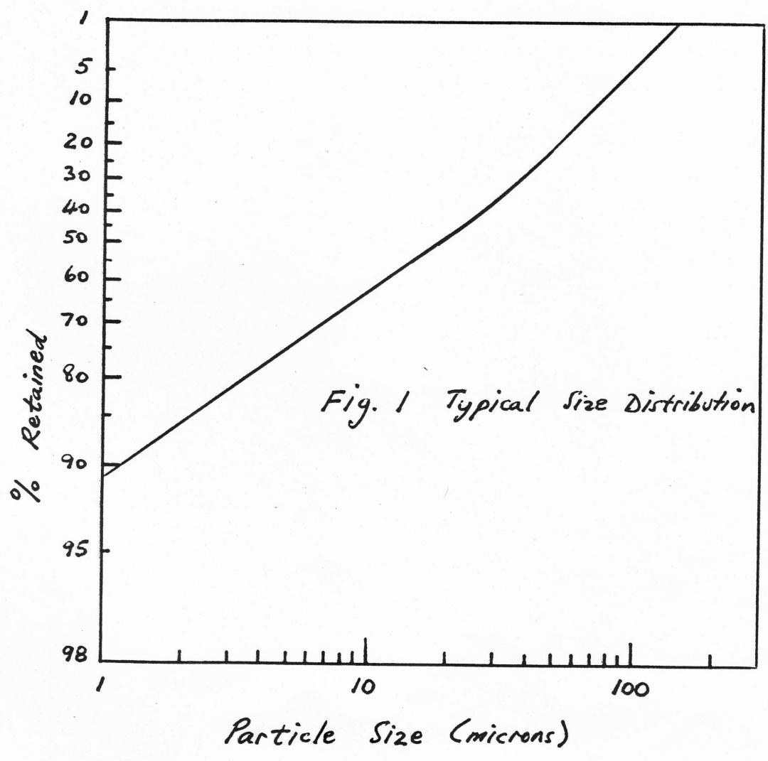
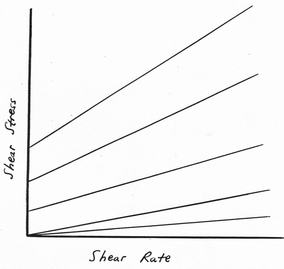
Shear Rate Fig 2. Typical Rheograms

Page 12

1000 100

Plastic Viscosity (mPus) Yield Stress (Pa)

→

Ll •1

10 20 40 60 80 100

Solids Concentration (%)

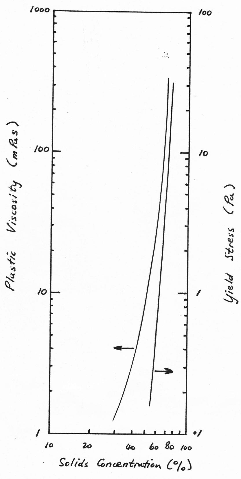
Fig. 3 Typical Rheology

Page 13

Pressure Gradient (KPalm)

• / •2 •4 • 6 •8 2 3 4 5

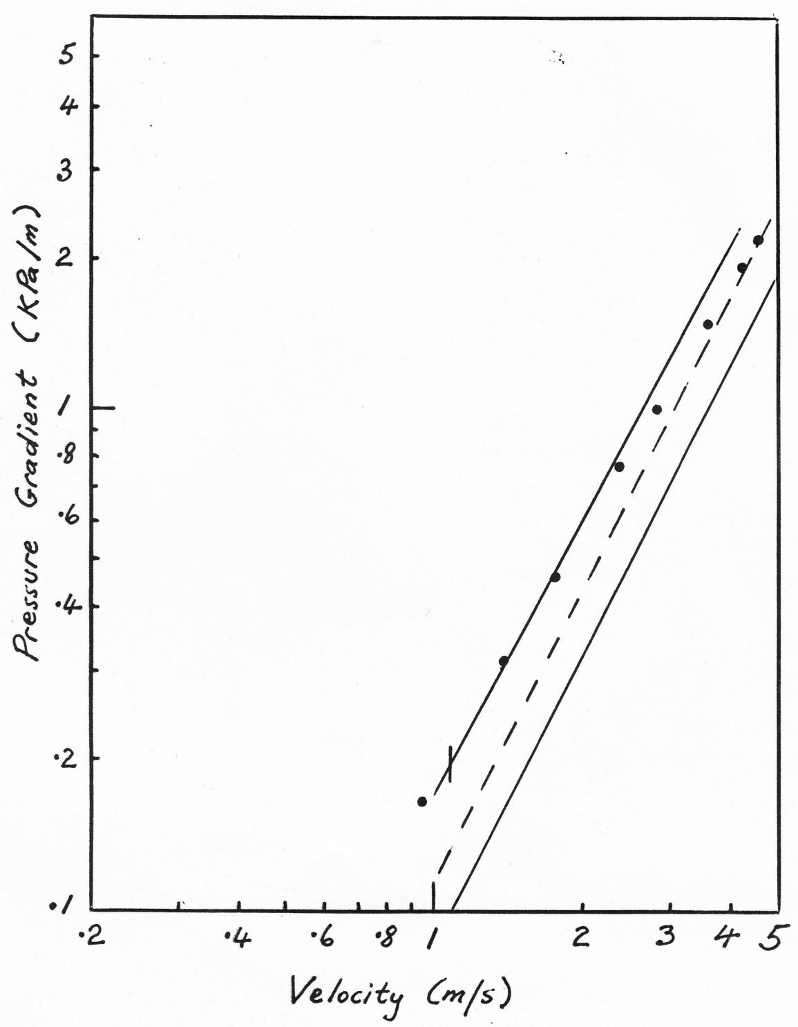
Velocity (m/s) • Fig. 4 Pipe hoop Resulte, 51%.

Page 14

4

15%

Pressure Gradient (KPa/m) 2 70% •

66%

Water

•2 •4 "6 2 3 4

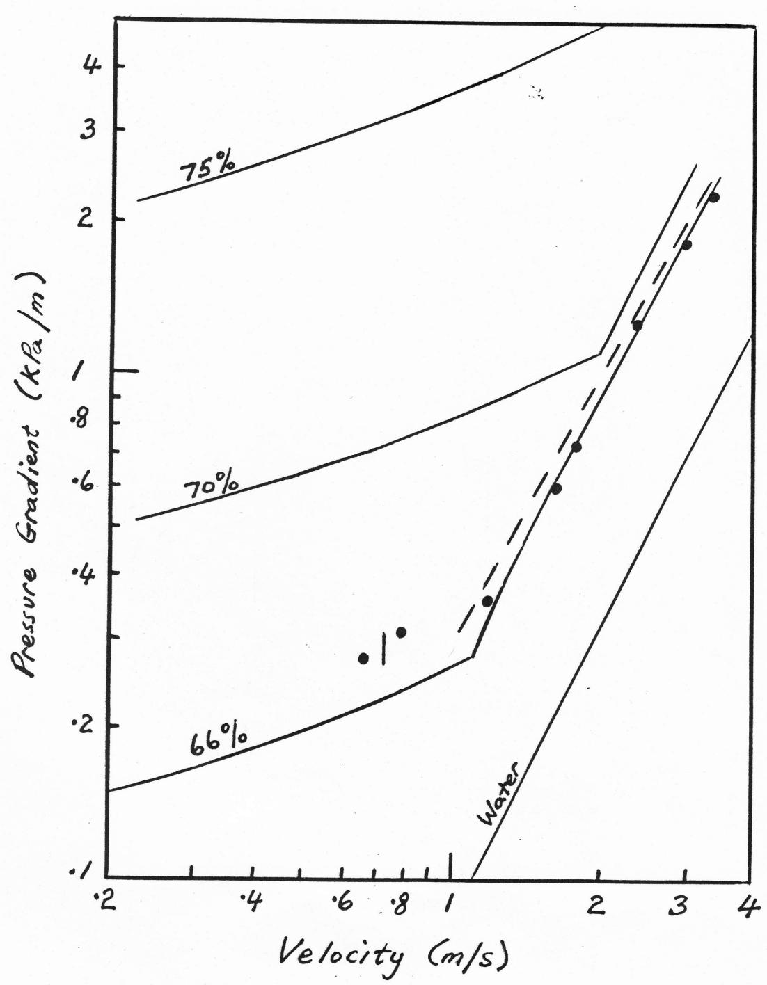
Velocity (m/s) Fig. 5 Pipe Loop Rerults, 66%.

Page 15

(KPa/m)

Pressure Gradient at 1.5 m/s

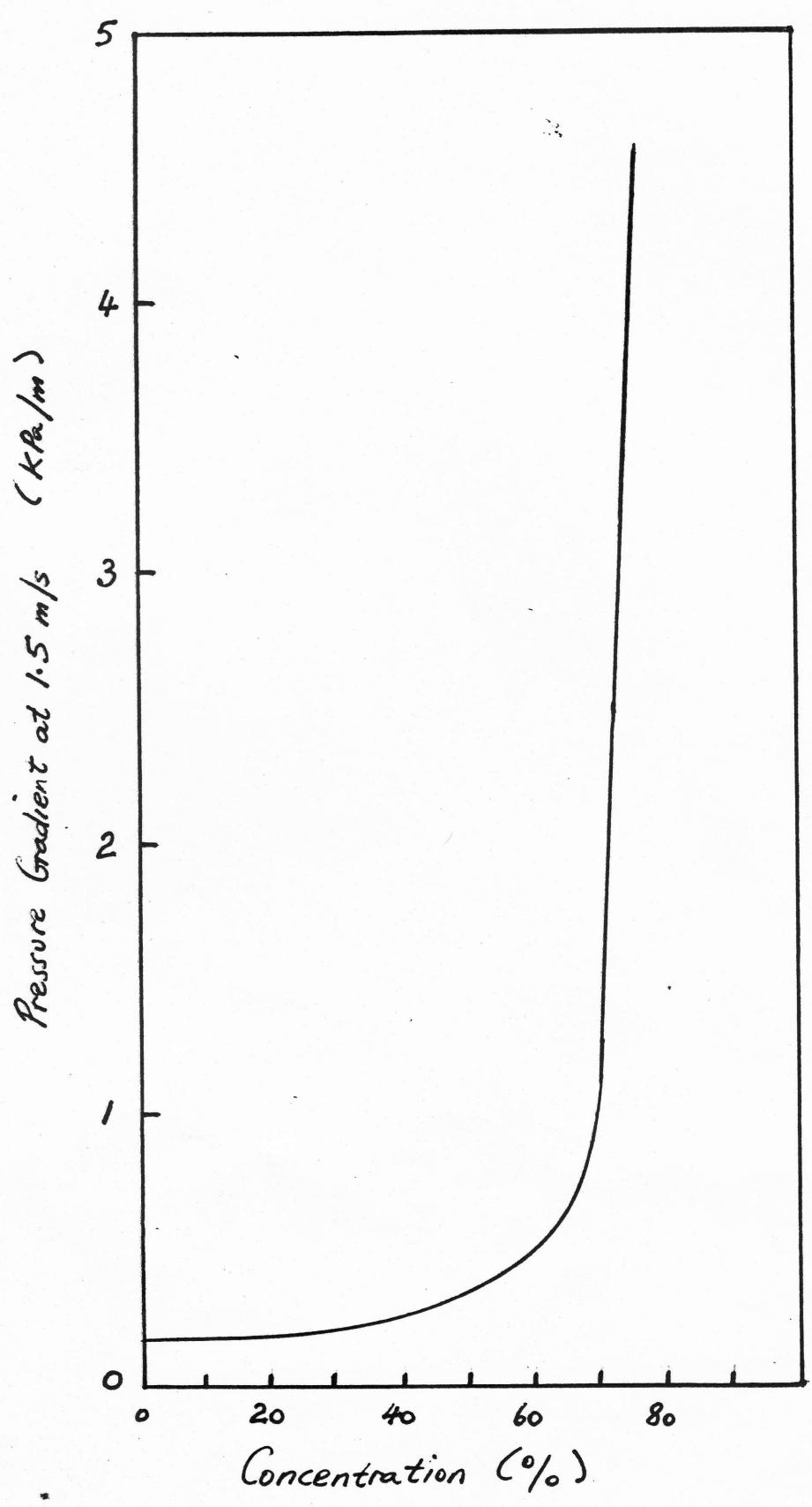
20 40 60 80 Concentration (%) Fig. 6 Pressure Gradient at 1.5m/s