On-line viscosity measurement for the mineral processing industry

ON-LINE VISCOSITY MEASUREMENT FOR THE MINERAL PROCESSING INDUSTRY

A. D. THOMAS N. T. COWPER P. B. VENTON

Slurry Systems Pty. Ltd.
Cammeray, N.S.W. 2062, Australia

1. INTRODUCTION

Mineral processing generally involves crushing and grinding of ore to release the valuable minerals. Although crushing is a dry process, water is usually added during grinding and from this stage on the various mineral processing steps involve slurry handling and pumping. Within the constraints of the various process requirements it is desirable that the slurry be as possible to minimise both the size of the equipment (capital cost) and pumping power (operating cost).

Slurry solids concentration is usually monitored by nuclear absorption density gauges and the various process steps are controlled using these density readings. As long as the ore remains uniform this is a satisfactory method of control. However with the inevitable trend towards lower grade and more difficult ores it is becoming increasingly apparent that density control is not sufficient to obtain maximum efficiency. There are a number of reasons, including:-

1. a) variations in the ore is low grade there is more gauge material present with the possibility of significant variations in its properties. This can result in considerable differences in viscosity for the same concentration.
2. b) Even some high grade ores may exhibit a large variation in viscosity and may have for this very reason been judged too difficult to mine in the past.
3. c) Low grade ore requires processing of much larger quantities of material. This makes it more imperative that the highest possible concentration be used.

In almost all process steps it is slurry viscosity and not solids concentration per se which is the limiting factor. The viscosity affects such such things as ball mill grinding performance, screen operation, cyclone performance, mixing and agitation, slurry thickening and slurry pumping. Continuous on-line viscosity measurement is an essential tool in increasing the future efficiency of all mineral processing plants, particularly those using chemical viscosity modifiers. Slurry Systems have developed an instrument which is robust and accurate, making process control by slurry viscosity a practical alternative to traditional control by density.

2. TRADITIONAL MINERAL PROCESSING

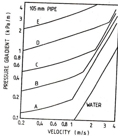
The traditional approach has been to operate at a conservative solids concentration such that any variations in slurry properties do not plant performance. This generally means operating equipment such that the flow is fully turbulent. Figure 1 illustrates the situation for pipe flow of a typical slurry. Such a slurry flow is shown in Figure 1. The lower sloping curve on the left represents the laminar flow portion whilst the steeply sloping curve on the right represents the turbulent flow regime. Transition between the two regimes occurs at 1 m/s. In the normal operating region between 1.5 to 2.5m/s flow is therefore turbulent. This slurry behavior would be typical of a traditional mineral slurry. As the slurry concentration is increased the behavior changes from a through to E. Between A and C there is about a 4 fold increase in the laminar pressure gradient but only about a 40% increase in the turbulent pressure gradient. Thus even large changes in viscosity have relatively little effect on the operating pressure gradient. However as the concentration is further increased from C to E, laminar flow now prevails in the operating velocity range. The operating pressure gradient now increases rapidly in direction to the viscosity. Operation in this region requires monitoring and control of the viscosity. Whereas once it was good enough to operate with slurry A with its large "factor of safety" up to slurry C without major effects on the plant performance, this is no longer the case. Increasingly there will be the need to operate continuously with slurry D in or near the laminar regime. Similar arguments apply to other process steps.

3. ON-LINE VISCOMETER REQUIREMENTS

A mineral processing plant presents an extremely harsh environment to any equipment. An on-line viscometer must be accurate, repeatable, and reliable, under all service conditions, requiring a robust design. With the present viscometer this robustness is achieved by keeping the instrument as simple as possible and by using well proven components which are already used extensively in the industry. The instrument must not clog in service and

preferably self drain upon shutdown. Abrasive slurries can cause severe wear problems. The instrument design must minimise wear, and if wear occurs, it should be low cost and their replacement effected as simply and quickly as possible. There are two most common types of viscometers - tube viscometers and rotational viscometers. We chose the tube viscometer principle because of its inherent simplicity.

4. DESCRIPTION OF VISCOMETER AND PRINCIPLE OF OPERATION

The viscometer consists of a measuring tube in the shape of an inverted U mounted in the vertical plane. The pressure drop across this U section is measured by a differential pressure transmitter. The tappings are pressured to prevent a build up of solids. They are at the same elevation to eliminate static head from the velocity is around 0.5m/s. The vertical configuration means any solids segregation has minimal influence on the pressure drop.

A magnetic flow meter and a flow control valve are installed downstream of the measuring tube in a smaller diameter resistance tube. Because of the higher velocity in this resistance tube the flow is turbulent. As discussed previously the resistance under turbulent flow is relatively insensitive to viscosity changes. By appropriate choice of length of resistance tube the pressure drop over the measuring tube the total resistance can be made much larger than the pressure drop over the measuring tube section making the pressure drop over the measuring tube relatively insensitive to viscosity changes. Thus as the slurry viscosity alters, the flow through the instrument changes only slightly. Slurry is normally supplied to the instrument by tapping into the process stream and fluctuations in pressure at the tapping point also alter the flow through the instrument. The control valve is operated by a programmable controller to maintain constant flow through the instrument. The pressure drop is changed by a 1 programmable controller in pressure causes large changes in velocity under laminar flow conditions but under turbulent flow velocity varies only as the square root of pressure drop. Thus incorporation of the resistance tube means the flow is more inherently stable and it reduces the work required of the control valve. The control valve keeping the flow rate constant to suit the feed pressure and the slurry viscosity range. With the length valve resistance tube rate selected to measure the pressure drop is a direct indication of the apparent slurry viscosity. This instrument meets all the aforementioned criteria:-

• - It is simple
• - All components are well proven in the industry
• - It is self draining upon shutdown
• - There are no moving parts (except for the flexing of the control valve muscle)
• - Measuring tube wear is negligible due to the low velocity. The resistance tube may wear but can easily and replaced by replaced control valves of this type are renowned for their wear resistance. The sleeve is easily valved with work harder. Control valves of this type are calibrationed, it will only mean the control valve has to work harder.

5. WHAT DOES THE INSTRUMENT READ?

For a Newtonian fluid the pressure gradient over a straight length of pipe is given by:

$$\frac{\Delta P}{L}=32\mu \frac{V}{D^2}(1)$$

Where $\mu$ is the viscosity, $V$ is mean viscosity, and $D$ is the pipe diameter. Hence in a given instrument for a constant flow rate the viscosity is directly proportional to the pressure gradient. Multiplying the pressure transmitter signal by an appropriate factor will give an instrument read out directly in viscosity units. For a non-Newtonian fluid this readout represents the effective Newtonian viscosity at an apparent shear rate of 8V/D reciprocal and is entirely suitable for control purposes.

Consider the special case of a Bingham fluid which is often used to model slurry behavior. The pressure gradient is given by the following approximation to the Buckingham equation, valid at higher shear rates. Here $\eta$ is the plastic viscosity and ${\tau }_{\gamma }$ is the yield stress.

$$\frac{\Delta P}{L}=\frac{32\eta V}{D^2}+\frac{16}{3}\frac{{\tau }_{\gamma }}{D}(2)$$

It is not generally realized that for mineral slurries the ratio ${\tau }_{\gamma }/\eta$ is relatively constant over typical concentration ranges of interest. Assuming ${\tau }_{\gamma }/\eta =K$ then:

$$\Delta P/L={\tau }_{\gamma }(32{\text{ V/KD}}^2+16/3D)(3)$$

For a constant flow rate the term in brackets is therefore approximately constant and so the yield stress is directly proportional to the pressure drop. Hence for a Bingham plastic instrument can be calibrated to read out directly in units of yield stress. Obviously this is not strictly correct but if yield stress is commonly used to characterise slurry consistency in a particular industry then it may be a convenient method of presentation. Of course the control capability of the instrument is unaffected whether the read out is termed viscosity or yield stress.

6. THE EFFECT OF THE U BEND

The above considerations apply to a straight length of pipe. However, this instrument includes a 180 degree bend as well as a 90 degree bend upstream of the first tapping. Also for practical reasons the pressure tappings are large and will disturb the flow and result in additional pressure drop. White [1] determined experimentally that the increased resistance due to a bend is a function of the Dean number given by:

$$De=\text{Re}\sqrt{D/D_c}(4)$$

where $De$ is the Reynold's number and $D_c$ is the diameter of the bend centre line. Using his relationship it can be shown that for a given pipe size and constant velocity the pressure drop around the bend ( $\Delta P_b$ ) is given by:

$$\Delta p_b=K_b{\mu }^{1-n}{p}^n(5)$$

where $p$ is the density of the fluid and $K_b$ is a constant for a given pipe size velocity and bend radius. The exponent $n$ varies between 0 and 0.4. In any particular application the slurry density will only vary over a small range, typically about 15%. This fact, combined with the small value of $n$ means the influence of density can be ignored.

Approximating each pressure tapping as a dead tee the additional pressure drop due to the tappings can be shown (using [3]) to be directly proportional to viscosity. The pressure drop in the straight sections of pipe is similarly directly proportional to viscosity (equation 1). Hence the total pressure drop is given by two terms, the first directly proportional to viscosity and the second proportional to ${\mu }^{1-n}$ . By appropriate choice of insignificant so that the bend radius and the tapping geometry, the second term can be made relatively insignificant so that a good approximation the total pressure drop is directly proportional to viscosity.

All of the foregoing applies to Newtonian fluids. For non-Newtonian fluids information is sparse. Mashelkar and Devarajan [4] studied the flow of power low fluids through bends. Their analysis and data indicate the influence of the bend is somewhat greater than in the case of an equivalent Newtonian fluid. For a Bingham fluid Cheng [5] states that the losses in fittings, relative to that of a Newtonian fluid, increase with a decrease in Reynolds number and can be a factor of ten higher when the Reynolds number is low. But he uses a Reynolds number based on the plastic viscosity. If an effective Newtonian Reynolds number is used based on the Newtonian viscosity which would give the same pressure gradient in a straight pipe as the Bingham plastic, the factor will be much less. Data for the same instrument indicate the losses are similar to that predicted by an equivalent Newtonian viscosity approach.

7. ACTUAL PERFORMANCE

Figure 2 shows results of commissioning tests on a limestone slurry at a cement plant. It shows the indicated yield stress compared to that measured in the laboratory on a Contraves RM15 rotational viscometer. The on-line instrument is seen to be reading consistently about 5% low. The instrument calibration can simply be adjusted to expect for this so as to give the true reading. There is some scatter of the data but no more than would be most likely give a similar degree of scatter.

8. CONCLUSIONS

An on-line viscometer has been described. This robust instrument is designed to withstand the rigorous environment in mineral processing plants. For a Newtonian fluid analysis has shown that the output is essentially directly proportional to fluid viscosity. For a Bingham plastic the instrument displays the yield stress and has been shown to give readings in good agreement with laboratory data.

9. REFERENCES

1. 1. White, C.M. Proc. Roy. Soc., A123, 645 (1929)
2. 2. Austin, L.R. and Seader, J.D. A.I.Ch.E.Jnl,19,nl,85 (1973)
3. 3. Jamison, D.K. and Villemonte, J.R. A.S.C.E. Jnl of Hyd.Div, July (1971) p 1045.
4. 4. Mashelkar, R.A. and Devarajan, G.V. Trans Instn Chem Engrs 54, 100 (1976).
5. 5. Cheng, D.C.H. Proc Hydrotransport 1 Conf., BHRA, Cranfield, England (1970).

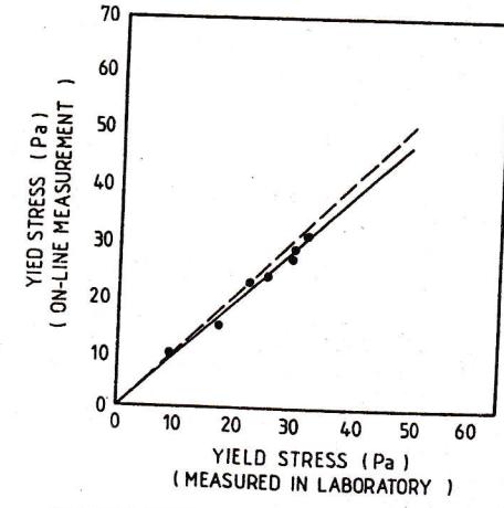
COMPARISON BETWEEN ON-LINE READING AND LABORATORY VISCOMETER READING

FIGURE 1

FIGURE 2