This HTML edition contains selectable text extracted from the original PDF. Layout-aware OCR was used to recover reading order, figures and equations; minor recognition errors may remain. Consult the PDF for the authoritative layout, figures and equations.
10th International Conference on Transport and
Sedimentation of Solid Particles
Wroclaw, Poland, Sept 2000.
A D Thomas
RELATIONSHIP BETWEEN VISCOMETER MEASUREMENTS AND
LAMINAR AND TURBULENT PIPE FLOW
Abstract
This paper considers the relationship between rheology measurements of slurry properties in a viscometer and the flow properties of the slurry in pipes under laminar and turbulent conditions. Selection of the most appropriate rheological model is discussed. The size of the particles relative to the relevant flow scale influences how the measured rheology relates to the observed shear stress or pressure gradient. Other factors of importance include the particle settling rate, the flow regime (laminar or turbulent), and orientation (horizontal or vertical).
NOTATION
| Symbol | Description | Unit |
|---|---|---|
| Volume concentration of solids | ||
| Maximum packing concentration | ||
| Pipe diameter | m | |
| Particle size | m | |
| Viscous sub-layer thickness | m | |
| Pressure gradient of clay slurry | Pa/m | |
| Pressure gradient of Newtonian fluid | Pa/m | |
| Pressure gradient of slurry | Pa/m | |
| Pressure gradient of water | Pa/m | |
| Fluid or slurry density | kg/m 3 | |
| Average velocity in pipe | m/s | |
| Friction velocity | m/s | |
| Viscosity of mixture | Pa.s | |
| Viscosity of fluid | Pa.s |
INTRODUCTION
The prediction of pipe flow behaviour of viscous slurries relies on rheology measurements generally made in a rotational viscometer. Relating the viscometer data to predicted pipe flow behaviour is not always straight forward. Some issues are: selecting the best rheological model; the effect of coarse particles on viscometer readings; allowing for the effect of coarse particles in laminar and turbulent pipe flow predictions; and the effect of particle settling on pipe flow predictions. These issues will be considered in turn.
LINEAR AND LOGARITHMIC RHEOGRAMS
A rotational viscometer is ideal for testing fine particle slurries. To obtain meaningful shear stress versus shear rate data ideally the gap between the bob and cup should be as small as possible. The Contraves viscometer used by the author has a gap width of 1.27 mm in the two bob and cup systems most frequently used. Fine particle slurries can be expected to give reliable data when tested in such a viscometer.
Figure 1 shows typical rheograms for fine particle slurries of low rheology. The lead concentrate has a top size of 50 microns and a size of 20 microns. The equivalent sizes for the Nickel Ore are 100 and 15 microns. Both slurries are sufficiently fine such that settling was not a significant problem during the viscometer tests.
The lowest data set (A) apply to a lead concentrate slurry at a solids concentration of 34.56% by weight. A straight line fits the majority of the data points. This indicates the Bingham Plastic model applies (Yield Stress 0.72 Pa, Plastic Viscosity 6.66 mPas). However for shear rates above 300 the three highest data points exhibit increasing deviation from the straight line data fit. This is due to the onset of Taylor vortex flow caused by inertial effects. The Taylor vortex data points can be easily identified on a linear plot of shear stress versus shear rate and should be disregarded.
The identification and rejection of data points caused by Taylor vortex flow is very important when testing low rheology slurries. For example most of the popular, less expensive commercial viscometers currently available will have problems if testing Slurry A because most of the data points will be affected by Taylor vortex error.
Data set B in Figure 1 applies to the same lead concentrate at a higher concentration of 37.49%. Once again the majority of the data points are fitted by a straight line giving the Bingham Plastic parameters Yield Stress 2.17 Pa and Plastic Viscosity 4.54 mPas. However the lowest shear rate data tend to fall below the straight line fit. Once again the highest shear rate data (in this case the two highest points) indicate Taylor vortex flow and are disregarded.
Data set C (nickel ore at 21.24% concentration) exhibits different behaviour from the other two slurries. The nickel ore slurry is sufficiently viscous such that Taylor vortex flow is not present over the measured shear rate range so all high shear rate data are relevant. However considerable deviation from a straight line fit is evident at shear rates below about 150 .
Figure 2 shows the same data as in Figure 1 plotted on logarithmic co-ordinates. The high shear rate data disregarded in Figure 1 due to Taylor vortex flow are not included in Figure 2. Figure 2 indicates that a straight line can be fitted to the four lowest shear rate data points for Set A, to the five lowest for Set B, and to the seven lowest for Set C. i.e. the low shear rate data which deviate most from the Bingham Plastic fit in Figure 1 are best fitted by a straight line on logarithmic co-ordinates. Conversely the high shear rate data which deviate from the straight line fit in Figure 2 fit the Bingham model in Figure 1. The straight lines fitted to the low shear rate data in Figure 2 apply to the Power Law model.
Figures 3 and 4 show rheological data for a backfill paste. The top size is 300 microns and the is 100 microns. Limitations apply when testing this very viscous material due to viscometer torque limits. As a result the maximum shear rates are less than in Figures 1 and 2. Although the high shear rate data in Figure 3 are fitted by a Bingham Plastic model (Yield Stress 29 and 49 Pa, and Plastic Viscosity 150 and 300 mPas) the Power Law model provides a much better fit over all of the shear rate range tested as evident in Figure 4.
For each slurry in Figures 1 to 4 a more complicated three parameter model such as the Yield Power law model may fit the entire data range better but the author's experience is that this added complexity is generally not required. The reasons are explained below.
SHEAR RATE RANGE OF INTEREST DETERMINES BEST RHEOLOGICAL MODEL
The shear rate range of interest determines whether the Bingham Plastic or Power Law model is most appropriate.
For pipeline transport of slurries, economic optimisation of capital costs versus operating costs dictate an operating velocity typically in the range 1 m/s to 1.75 m/s unless the particles are so coarse as to require a higher operating velocity to avoid deposition. Long distance slurry pipelines generally operate in turbulent flow meaning that the laminar-turbulent transition velocity must be below the operating velocity. Since solids throughput is required to be maximised it is desirable to operate at a solids concentration as high as possible. This means that the transition velocity will generally be just below the operating velocity at around 1 m/s.
Figure 5 shows the predicted behaviour of the 37.49% concentration lead concentrate in a 300 mm NB pipe. The prediction is based on the Bingham Plastic parameters from the straight line fit to the high shear rate data in Figure 1 (Yield Stress 2.17 Pa, Plastic Viscosity 4.54 mPas). The laminar flow prediction is based on the well known Buckingham equation. The turbulent flow prediction uses the theory of Wilson and Thomas (1985). The predictions are shown in terms of wall shear stress versus apparent shear rate (8V/D where V is the velocity and D is the pipe diameter). The wall shear rate range shown in Figure 5 equates to a pressure gradient range of 33 kPa/km to 103 kPa/km. The apparent shear rate range shown equates to a velocity range of 0.55 m/s to 1.75 m/s. Transition occurs at an apparent shear rate of 27 sec -1 equivalent to a velocity of 1 m/s.
The minimum wall shear stress in Figure 5 is 2.5 Pa. Comparison with rheogram B of Figures 1 and 2 shows that the Bingham Plastic model is most appropriate for shear stress values above 2.5 Pa. In Figure 5 the wall shear stress under turbulent flow conditions ranges from 2.6 Pa to 7.7 Pa. For this shear stress range the Bingham Plastic model is most appropriate and is used to predict the turbulent flow pressure gradient.
The paste backfill data shown in Figures 3 and 4 are examples of high rheology slurries. The data relate to a system involving a 250 mm NB pipe with a maximum design velocity of 1.15 m/s. The apparent shear rate (8V/D) is 37 sec -1 and the true shear rate is around 45 sec -1 . Figure 3 indicates that the Bingham Plastic model only applies for shear rates above about 100 sec -1 and is not appropriate for the design shear rate of 45 sec -1 . The Power Law model is the most appropriate for a shear rate of 45 sec -1 as seen in Figure 4. At the design velocity of 1.15 m/s the paste flows laminarly. Transition to turbulent flow does not occur until far higher velocities.
In summary, for low rheology slurries which flow under turbulent flow conditions in the economic velocity range of 1 to 1.75 m/s, the viscometer data is generally best analysed using the Bingham Plastic model. High rheology slurries which flow under laminar flow conditions in the normal velocity range are generally best analysed using the Power Law model.
VISCOMETER WALL INTERFERENCE EFFECTS WITH COARSE PARTICLES
The slurries considered thus far all consist of fine particles with a wide size distribution. Slurries containing a greater proportion of coarser particles can cause problems during viscometer tests due to mechanical wall interference effects artificially increasing the measured shear stress. This latter effect means that the measured shear stress in the viscometer may overestimate the shear stress in a pipe where interference effects are not so relevant due to the much larger ratio of pipe diameter to particle size.
An often quoted rule of thumb is that the viscometer gap size should be at least 10 times the maximum particle size. The author believes this limit is too stringent and that meaningful results can be obtained with much coarser material with a gap to maximum particle size ratio as small as 2.5 at least at low concentrations.
Interference effects due to crowding of coarse particles in the narrow gap of a viscometer can be expected to depend both on the particle size to gap ratio and on the volume concentration of solids. i.e. low concentration of coarse particles may cause minimal interference whereas high concentration of the same size particles may cause significant interference effects.
A brief investigation into the phenomenon has been conducted. Viscometer tests were performed with a bob and cup system having a 1.27 mm gap. Two different size sands were tested at a number of concentrations. The sand samples were obtained by screening to produce a 0.30 mm x 0.18 mm sand (mean size 0.24 mm) and a 0.60 mm x 0.425 mm sand (mean size 0.51 mm). The respective gap to mean size ratios are 5.3 and 2.5. The sands were tested in Sodium Silicate fluid of SG 1.38 and Newtonian viscosity 32 mPas. The SG of the sand was 2.64.
The 0.24 mm sand was tested at three volume concentrations 12.5%, 23.2%, and 39.2%. The 0.51 mm sand was tested at two volume concentrations 16.0% and 24.6%. In each case tests were conducted over a range of shear rates and straight lines passing through the origin fitted to obtain the Newtonian viscosity and the results expressed as a ratio of the fluid viscosity.
The results are presented in Figure 6. The full line curve in Figure 6 is the predicted relationship due to Landel et al (1963).
| where | = | viscosity of mixture | |
| = | fluid viscosity | ||
| = | Volume concentration of solids | ||
| = |
Maximum packing concentration
(Assumed = 0.75) |
Thomas (1999) presented data from the literature (Thomas 1978, 1979/2 and Shook et al 1973) for laminar flow of narrow size distribution sands in high viscosity fluids in pipes. The data was found to be adequately described by Equation 1. The ratio of pipe diameter to particle size ranged from 128 to 800 so wall interference effects would be expected to be negligible.
The gap to particle size ratio in the present viscometer tests (Figure 6) is much smaller (5 and 2.35) and yet Equation 1 still appears to describe the data at least at low concentrations. Figure 6 suggests that Equation 1 describes the 0.24 mm sand (gap to sand ratio 5.3) results for volume concentrations up to about 25% and describes the 0.51 mm sand data (gap to sand ratio 2.5) for volume concentrations up to about 15%.
The present viscometer tests are by no means comprehensive. Also particle settling during testing was a problem and resulted in a large degree of scatter. Nevertheless the results do suggest that meaningful results can be obtained from viscometer tests in which the gap to particle size ratio is as small as 2.5.
Figure 6 applies to sand in a Newtonian fluid. Thomas (1999) showed that Equations analogous to Equation 1 described the effect of sand addition on the Yield Stress and Plastic Viscosity of colloidal slimes slurries. The present findings suggest that coarse particle slurries can be successfully characterised even if the gap to particle size ratio is as small as 2.5. However in cases where the gap size to particle size is very small care is needed if testing at high concentrations. The measured rheology may be higher than the true rheology due to interference effects. If a problem is suspected tests should be conducted at a number of lower concentrations and the rheology extrapolated to higher concentrations using for example equations given by Thomas (1999), rather than use the measured rheology at high concentrations.
APPLYING VISCOMETER DATA TO LAMINAR AND TURBULENT PIPE FLOW PREDICTION
The effect of coarse particles on viscometer test results was discussed above. The question of how the resulting measured rheology should be applied to laminar and turbulent pipe flow prediction will now be considered.
If the slurry is sufficiently viscous and/or sufficiently fine and of low solids SG the laminar flow pressure gradient should be directly predicted based on the measured rheology. However an interesting complication arises when predicting turbulent flow pressure gradient.
Durand (1953) was among the first to observe that the pressure gradient in vertical pipe flow of coarse particles in water was similar to the pressure gradient for water flowing alone. This was also observed by Newitt et al (1961) and Toda et al (1969). A similar effect was observed with the flow of neutrally buoyant particles in water in a horizontal pipe by Dailey and Roberts (1965).
The phenomenon is associated with the fact that the coarse particles are larger than the viscous sublayer. Very fine particles, much smaller than the viscous sublayer, will reside within the sublayer and increase the viscosity in the wall region. In contrast very coarse particles are not able to reside within the sublayer meaning that the relevant viscosity in the wall region is that of water. Wilson et al (1992, pp 107-110) discuss this phenomenon in some detail.
Data for sand of various particle sizes in Newtonian fluids was analysed by Thomas (1977/1) and his results are reproduced here in Figure 7. Figure 7 shows the ratio of slurry pressure gradient to fluid pressure gradient at the same velocity ( ) versus the ratio where is the particle size and is the thickness of the viscous sublayer given by:
The data in Figure 7 apply to sand slurries of narrow particle size distributions flowing at sufficiently high velocities such that heterogeneous settling effects have negligible contribution to the pressure gradient. Data for volume concentrations of 12% and 30% are shown taken from experimental results obtained by the author and by Shriek et al (1973) and Shook et al (1973).
Figure 7 suggests that for coarse particles much larger than the viscous sublayer ( ) is around 1.07 as proposed by Murphy et al (1955). As the particle size reduces and becomes less than 3 the ratio increases up to a value consistent with a homogeneous slurry with density and viscosity increased due to the solids. Assuming the friction factor varies roughly with Reynolds Number to the power for the pipe sizes and velocities considered, will increase as slurry density ratio to the power 0.8 times slurry viscosity ratio to the power 0.2.
For a volume concentration of 12% equation 1 indicates a viscosity ratio of 1.55. In the case of sand in water the density ratio is 1.20. The predicted pressure gradient ratio for homogeneous flow of fine particle sand in water is:
This is consistent with the results shown in Figure 7 at low ratios. A similar calculation for a volume concentration of 30% gives:
Once again this is supported by the data of Figure 7 at low ratios.
The differing behaviour of coarse and fine particles would be expected to similarly occur in the case of turbulent flow of coarse particles in a non-Newtonian vehicle slurry. Thomas (1978) presented data for both coarse and fine sand and coarse and fine coal in a clay vehicle slurry which supported this expected behaviour. The consequences for pipe flow prediction are illustrated by Figure 8 which shows data for fine and coarse coal in a clay slurry taken from that early work. The data apply to a minus 1 mm coal of median size 0.44 mm slurry taken from that early work. The data apply to a minus 1 mm coal of median size 0.44 mm slurry taken from that early work. The solids SG of the coal was 1.31 and the SG of the kaolin clay slurry was 1.11 so there was not a large relative SG difference. This meant that even the coarse coal slurry could flow in laminar flow without significant settling at least in the length of the test loop. At high shear rates the clay vehicle slurry approximated a Bingham Plastic with a Yield Stress of 5 Pa and a Plastic Viscosity of 4.5 mPas.
Figure 8 shows measured pressure gradient versus velocity for water, clay alone and the fine and coarse coal slurries at a coal volume concentration of 20%. Below about 2 m/s both coal slurries flowed in laminar flow and the pressure gradients are similar at approximately twice the pressure gradient of the clay alone. This pressure gradient increase is consistent with a viscosity increase of about 2 shown in Figure 6 for a volume concentration of 20%.
At velocities above 2 m/s turbulent flow occurs but with significantly different pressure gradients for the fine and coarse coal. The different behaviour is consistent with the effect discussed above. At a velocity of 2 m/s, just above transition, the calculated thickness of the viscous sub-layer is 1.85 mm after allowing for the thickening of the viscous sub-layer as proposed Wilson and Thomas (1985). All of the minus 1 mm fine coal is less than 1.85 mm and Figure 7 indicates that the pressure gradient ratio should be given by the homogeneous pressure gradient increase. For viscous slurries such as this it is reasonable to assume that the friction factor varies as Reynolds Number to the power . The density ratio of coal slurry to clay slurry is 1.122 and the viscosity ratio for 20% volume concentration from equation 1 is 2.17. On this basis the pressure gradient ratio at 2 m/s for the fine coal slurry should be approximated by:
The actual pressure gradient ratio at 2 m/s for the fine coal is 1.42.
For the minus 10 mm coarse coal only 40% of the particles are less than the 1.85 mm viscous sub-layer thickness at 2 m/s. This suggests that the pressure gradient ratio for the coarse coal will be less than the homogeneous ratio given by Equation 5. The actual pressure gradient ratio at 2 m/s for the coarse coal is 1.29.
Although the actual pressure gradient ratios for the two coals are somewhat higher than predicted the data do indicate the correct trends, namely the fine coal is exhibiting homogeneous fluid behaviour whilst the coarse coal is exhibiting some reduction due to effects.
As the velocity increases the pressure gradient of the minus 10 mm coal approaches that of the clay alone. At 3.5 m/s the calculated value for is 0.46 mm. Almost all (95%) of the minus 10 mm coal is coarser than 0.46 mm which is consistent with the observed pressure gradient at 3.5 m/s being similar to that of the clay alone. Approximately 50% of the minus 1 mm coal is less than 0.46 mm so the pressure gradient ratio of the fine coal is still substantially above that of the clay alone. The observed pressure gradient ratio decreases from 1.42 at 2 m/s to 1.18 at 3.5 m/s. This is consistent with the change in the proportion of particles less than the viscous sub-layer from 100% at 2 m/s to 50% at 3.5 m/s.
The above consideration of the behaviour of fine and coarse coal transported in a clay slurry suggests the following:
- • Measured rheology obtained in a viscometer can be used directly to predict laminar pipe flow behaviour for any size particles provided any influence of particle size effects in the viscometer gap has been addressed.
- • For a fine particle slurry where all particles are finer than the expected viscous sub-layer thickness the measured rheology can be used to predict the turbulent pressure gradient.
- • For a coarse particle slurry where some or all of the particles are coarser than the expected viscous sub-layer thickness, then use of the measured rheology will over-predict the pressure gradient. An accurate prediction of the turbulent flow pressure gradient needs to take into account viscous sub-layer effects analogous to Figure 7.
In reality most slurries have a continuous particle size distribution rather than a distinct "coarse" component in a much finer vehicle slurry component. In this case the question arises as to what can be considered the "vehicle" portion of the slurry. This question cannot be easily answered.
Interestingly, however, given that a typical viscometer gap size is of roughly the same order of magnitude as the size of the viscous sub-layer, rheology tests on a screened portion of a coarse particle slurry would seem directly relevant to turbulent pressure gradient prediction. i.e. suppose a viscous coarse particle slurry is to be tested in a viscometer to enable prediction of the laminar and turbulent
pipe flow behaviour. The slurry might be screened at say 0.5 mm with only the minus 0.5 mm material tested in the viscometer. Since the plus 0.5 mm fraction is likely to be larger than the viscous sub-layer thickness it will not contribute to the turbulent pressure gradient. Thus, to a first approximation, the rheology and density of the minus 0.5 mm fraction tested in the viscometer are the appropriate quantities to use in predicting turbulent flow pressure gradient for the total slurry.
For example, if a coarse particle slurry is to be pumped at say 30% by volume and half of the particles are coarser than 0.5 mm and are screened out before viscometer tests, then the rheology and density of the tested portion (volume concentration 18%) can be used directly to predict an approximate turbulent flow pressure gradient. The plus 0.5 mm material is in effect transported for free. In contrast the plus 0.5 mm particles will contribute to the relevant rheology for laminar flow prediction and the measured rheology of the minus 0.5 mm fraction will need to be increased accordingly, using for example the methods given by Thomas 1999.
PARTICLE SETTLING EFFECTS
The above discussion on laminar and turbulent flow pressure gradient prediction has not considered the effect of particle settling. If the Yield Stress of a slurry is sufficiently high the floc structure will prevent the coarsest particles settling under static conditions as explained by Thomas (1977/2). However once the slurry is subject to laminar shear the floc structure is broken and settling of the coarsest particles can occur. In a rotational viscometer the settling is transverse to the direction of primary shear. Settling under these conditions has been studied for example by Thomas (1979/1) and Wilson (1998).
In horizontal laminar pipe flow a similar settling tendancy occurs. If the settling tendancy is high the coarser particles will be transported as a saltating/sliding bed analogous to pipe flow of very coarse particles in water. In the case of heterogeneous turbulent flow some of the particles may be supported by turbulent eddies. In the laminar flow situation there is no turbulent support available. There may be some "off the wall" force present due to velocity profile effects which may help suspend particles but this force has not yet been fully identified.
The possibility of settling under laminar flow in a horizontal pipeline introduces uncertainty into pressure gradient prediction based on viscometer data. For example the predicted laminar flow curve for the lead concentrate shown in Figure 5 cannot be guaranteed to represent the actual laminar flow behaviour in horizontal pipe flow. In fact for the particle size, solids SG, and rheology conditions too low. The actual laminar flow pressure gradient curve predicted from viscometer data shown is too low. The actual laminar flow pressure gradient is higher due to heterogeneous settling effects. The intersection of the predicted laminar and turbulent flow curves can be used to predict the transition point but the predicted laminar flow curve cannot be guaranteed relevant. It is well known that settling effects in vertical pipe flow are much less significant than in horizontal pipe flow. The laminar flow prediction in Figure 5 is applicable to vertical pipe flow.
The relationship between the degree of settling in a viscometer and in a horizontal pipeline is not yet quantified. The observation of very little settling occurring during viscometer tests is no guarantee that settling will not occur in pipe flow. The reason why settling is more likely to occur in pipeline flow is that settling tendancy involves a scale effect over and above that allowed for by wall shear stress. For example viscometer tests without significant settling could be conducted on a slurry at shear stress values similar to those expected for laminar flow of the slurry in a pipe. But this is no guarantee that the same slurry will flow under laminar flow conditions at the same wall shear stress without settling in a pipeline. Thomas (1979/2) showed how successful laminar flow of a slurry in a 18.9 mm diameter pipe did not guarantee that the same slurry could flow under laminar flow conditions without settling in a larger 105 mm diameter pipe. A similar situation applies when trying to extrapolate viscometer data to large pipe flow because of the different size scales involved.
Pipeline length is also an important parameter in regard to settling under laminar flow conditions. This was first investigated by Thomas (1979/2). A fine particle slurry flowing laminarly in a pipeline of length say 1 km may not exhibit noticeable settling and pressure increase whereas the same slurry in a pipeline of say 100 km showed long settling and pressure increase. A recent paper by Aude et al (1996) considered settling and resultant pressure gradient increase in three long distance
slurry pipelines operating in laminar flow and found that even quite fine particle slurries (particle size less than 300 microns) settled over long distances.
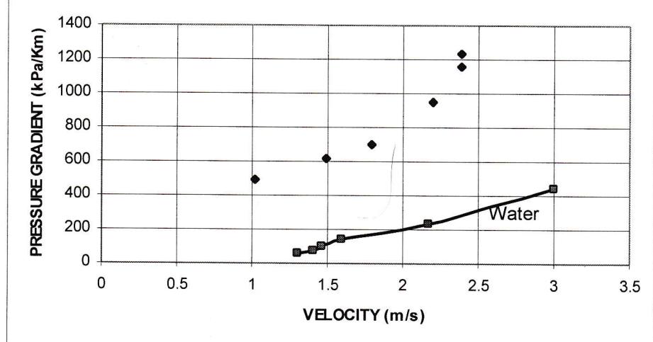
The reality is that some settling will generally occur under laminar flow in a horizontal pipe unless the slurry consists of all colloidal sized particles or the relative density difference between the coarse particles and the "vehicle" portion is low. If granular material of high solids SG is present then settling will generally occur even if the slurry is very viscous. Figure 9 shows data obtained in a 146 mm ID pipe. The slurry is backfill tailings at a concentration of 71% by weight. Maximum particle size is 300 microns and the median particle size is 85 microns. Solids SG is 3.28. The test facility consisted of a once through pipe of length 200 m. A transparent viewing spool was located at 180 m. The two data points at the highest velocity of 2.39 m/s were clearly in turbulent flow and no bed of solids was present. At 2.2 m/s transition flow was observed with a laminar flow generally present but with regular turbulent bursts. Solids were flow was observed during the laminar flow periods and then be picked up as a turbulent burst passed through. At a velocity of 1.79 m/s and below laminar flow was present. At 1.79 m/s a stationary bed of solids occupied 1/5 th of the pipe diameter. At a velocity of 1 m/s the bed height had increased to about 1/3 rd of the pipe diameter.
Figure 9 illustrates how settling can occur under laminar flow conditions even though the slurry is relatively viscous and the pressure gradient is high. This slurry had a Yield Stress of 25 Pa and is approaching the maximum consistency able to pumped using a centrifugal pump and yet laminar flow without deposition is not possible in this size pipe.
At this stage there is no published method available to predict the degree of settling in laminar flow pipelines and its effect on pressure gradient. Development of a prediction method will involve combining a sliding bed analysis, particle settling rates in a Bingham Plastic, and possible "off the wall" lift force effects. Obviously settling is less likely to occur with a combination of a high Yield Stress slurry, fine particles, low solids SG, small pipe diameter and short pipeline length. The key to a prediction method is the sliding bed analysis such as developed by Wilson over a number of years. See for example Wilson et al (1992). In the absence of turbulent support the sliding bed model requires a certain pressure gradient to transport the bed load solids. The same will apply in a laminar flow settling situation. i.e. a certain critical pressure gradient is required to prevent settling under laminar flow conditions. This explains why a slurry can flow laminarly in a small diameter pipe without settling but settling will occur in a larger size pipe. For homogeneous flow the pressure gradient decreases as the pipe size increases. If the "homogeneous" pressure gradient is less than the critical pressure gradient required to prevent settling then settling will occur.
TRANSITION FROM LAMINAR TO TURBULENT FLOW
There has been considerable debate over the years about whether the transition between laminar and turbulent flow is a sharp transition or occurs over a significant velocity range. The author's experience is that for slurries consisting of all colloidal particles e.g. a clay slurry, the transition is generally quite sharp on a plot of pressure gradient versus velocity. In contrast many wide particle size distribution slurries slurries having a combination of colloidal and coarse particles, often exhibit a more gradual transition from the turbulent flow pressure gradient curve to the laminar flow pressure gradient curve which may be thought of as an extended transition region. It is of interest to note that two of the phenomenon discussed in this paper could contribute to an "extended transition region".
The d/ effect illustrated in Figure 8 results in a gradual decrease in the ratio of coarse coal slurry pressure gradient to clay pressure gradient as the velocity increases from say 2 m/s to 3 m/s. This could be construed as an extended transition region.
Similarly settling effects in the transition and laminar flow regions could result in a more gradual change from the turbulent pressure gradient plot to the laminar plot than would be expected. For example a particular slurry may flow without any settling tendancy under turbulent flow. However as the velocity is reduced and transition begins some settling may occur resulting in either a moving or fixed bed. The velocity above the bed increases meaning that the flow is still in the transition region above the bed even though the superficial velocity may be further reduced. The result is an apparent extended transition region caused by settling. This effect will be particularly relevant to test loop situations where the volume of the pipework is significant compared with the feed tank volume and if insufficient time is allowed for equilibrium conditions to be achieved. If the feed tank volume is
relatively large and sufficient time is allowed for equilibrium conditions to be achieved the concentration above the bed will be at the feed concentration and the pressure gradient may in fact rise as the flow rate is reduced. If this occurred it would be recognised as a heterogeneous situation rather than an extended transition region.
CONCLUSIONS
Rotational viscometer tests on fine particle slurries can be used to predict pipeline pressure gradient. In general the Bingham Plastic model fitted to high shear rate data is appropriate for low rheology slurries for which turbulent flow behaviour is of interest whilst the Power Law model is more appropriate to high rheology slurries where laminar pipe flow behaviour is of interest.
With coarse particle slurries relevant rheology can be obtained in a viscometer even in cases where the ratio of gap width to particle size is as small as 2.5. The measured rheology obtained in a viscometer can be used directly to predict laminar pipe flow behaviour for any size particles provided any influence of particle size effects in the viscometer gap has been addressed.
For a fine particle slurry where all particles are finer than the expected viscous sub-layer thickness the measured rheology can be used to predict the turbulent pressure gradient. For a coarse particle slurry where some or all of the particles are coarser than the expected viscous sub-layer thickness, then use of the measured rheology will over-predict the pressure gradient. An accurate prediction of the turbulent flow pressure gradient needs to take into account viscous sub-layer effects analogous to Figure 7.
Laminar flow predictions must consider the possibility of settling. At present there is no published method available to predict settling.
The extended transition region observed by some researchers may be associated with either the viscous sub-layer effect and/or settling effects.
REFERENCES
AUDE T C, DERAMMELAERE R H, and WASP E J (1996), Instability of laminar flow in long distance pipelines and solutions, 21st Int Tech Conf on Coal Utilization & Fuel Systems, March 18-21, Clearwater, Florida.
DAILY W D and ROBERTS P R (1969), Rigid particle suspensions in turbulent shear flow , Tappi, Vol 49, n3, pp 115-125.
DURAND R (1953), Basic relationships of the transportation of solids in pipes , Proc Minn Int Hydr Conv, Int Assoc for Hyd Res pp 89-103.
LANDEL R F, MOSER B G, and BAUMAN A J (1963), 4 th Int Congress on Rheology, Brown University, Proc. Part 2, pp663.
MURPHY G, YOUNG D F, and BURIAN R J, Progress report on friction loss of slurries in straight tubes , USAEC, Report ISC-474 (79p).
NEWITT D M, RICHARDSON J F, and GLIDDON G J (1961), Hydraulic conveying of solids in vertical pipes , Trans Instn Chem Engrs, Vol 39, pp 93-100.
SCHRIEK W, SMITH L G, HAAS D B, and HUSBAND W H W (1973), Experimental studies on the transport of two different sands in water in 2, 4, 6, 8, 10 and 12 inch pipes , Saskatchewan Research Council of Canada, Report E73-21.
SHOOK C A, SCHRIEK W, SMITH L G, HAAS D B and HUSBAND W H W (1973), Experimental studies on the transport of sands in liquids of varying properties in 2 and 4 inch pipelines, Report E73-20, Saskatchewan Research Council, Canada.
TODA M, KONNO H, SAITO S, and MAEDA S (1969), Int. Chem Engnr, Vol 9, n3, pp553-560.
THOMAS A D (1977/1), Particle size effects in turbulent pipe flow of solid-liquid suspensions , 6 th Australasian Hydraulics and Fluid Mechanics Conf., Adelaide, 5-9 Dec, pp 113-116.
THOMAS A D (1977/2), A rational design philosophy for long distance slurry pipelines , Chem Engng in Australia, Instn of Engnrs Aust, pp22-33.
THOMAS A D (1978), Coarse particles in a heavy medium-turbulent pressure drop reduction and deposition under laminar flow , Hydrotransport 5 Conf, Hannover, BHRA Fluid Engineering.
THOMAS A D (1979/1), Settling of particles in a horizontally sheared Bingham plastic , 1 st National Conference on Rheology, Melbourne, May, pp 89-92.
THOMAS A D (1979/2), Pipelining of coarse coal as a stabilized slurry – another viewpoint , 4 th Int Tech Conf on Slurry Transportation, March 28-30, Las Vegas.
THOMAS A D (1999), The influence of coarse particles on the rheology of fine particle slurries, Rheology in the Mineral Industry II, March 14-19, Turtle Bay, Hawaii.
WILSON K C and THOMAS A D (1985), A new analysis of the turbulent flow of non-Newtonian fluids , Can Jnl Chem Eng, Vol 63, Aug 1985, 539-546.
WILSON K C, ADDIE G R, and CLIFT R (1992), Slurry transport using centrifugal pumps , Elsevier.
WILSON K C (1998), Particle motion in sheared non-Newtonian media ,
FIGURE 1 TYPICAL RHEOGRAMS LOW RHEOLOGY SLURRIES
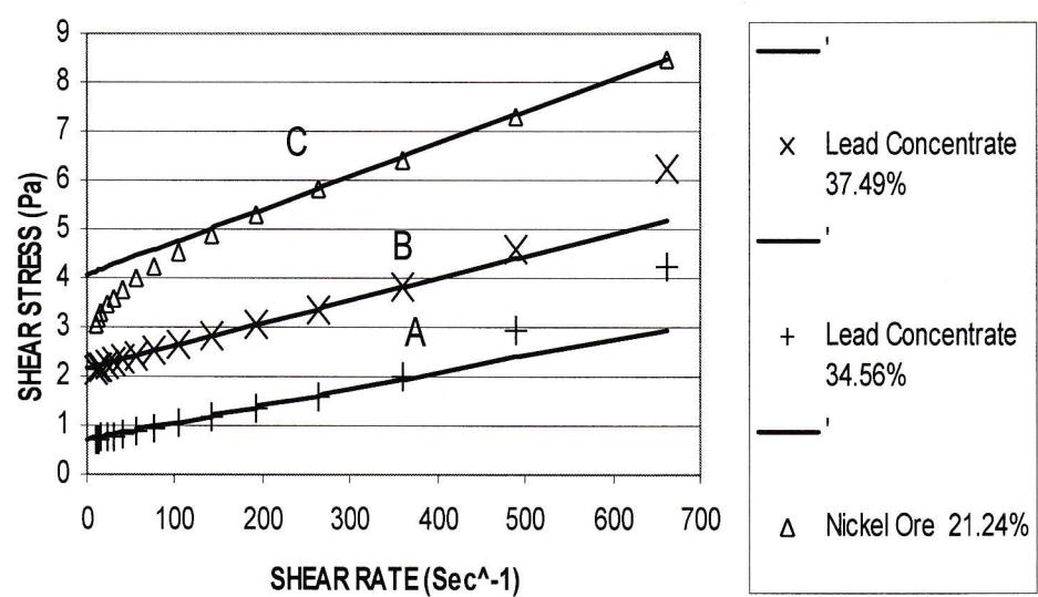
FIGURE 2 TYPICAL RHEOGRAMS LOW RHEOLOGY SLURRIES - LOGARITHMIC PLOT
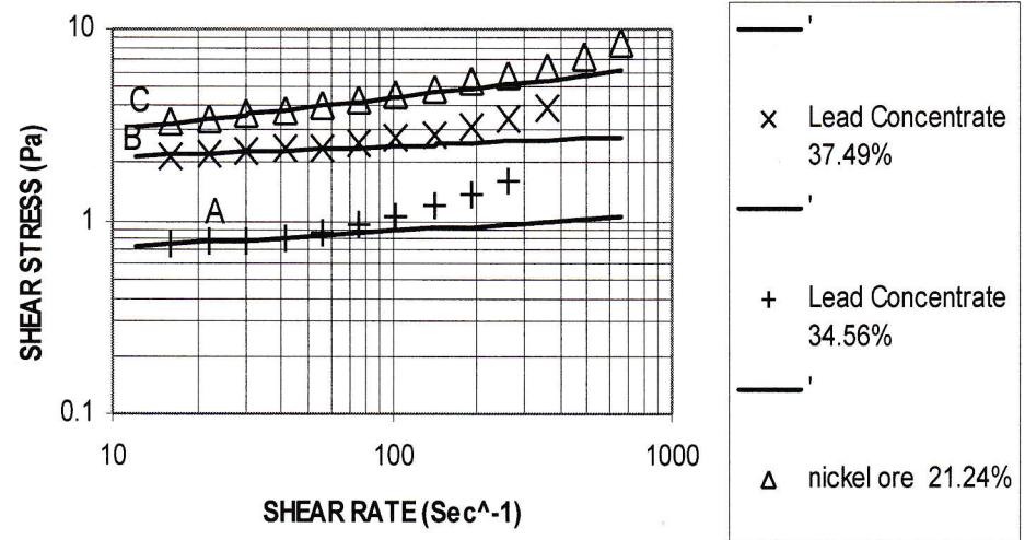
FIGURE 3 TYPICAL RHEOGRAMS HIGH RHEOLOGY SLURRIES
PASTE BACKFILL SLURRY
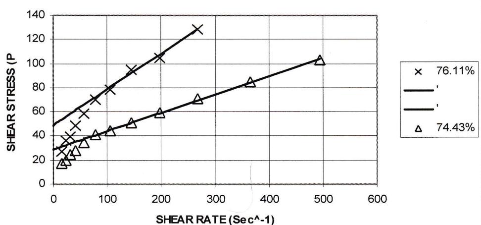
FIGURE 4 TYPICAL RHEOGRAMS HIGH RHEOLOGY SLURRIES
LOGARITHMIC PLOT
FIGURE 5 TURBULENT FLOW OF LOW RHEOLOGY SLURRY
LEAD CONCENTRATE 37.49% CONCENTRATION
300 MM NB PIPE
FIGURE 6 VISCOSITY INCREASE DUE TO COARSE PARTICLES SAND IN NEWTONIAN FLUID 1.2 MM VISCOMETER GAP
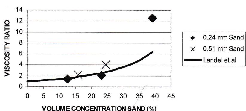
FIGURE 7 VISCOUS SUB-LAYER EFFECTS TURBULENT FLOW OF SAND IN NEWTONIAN FLUIDS FROM THOMAS (1977/1)
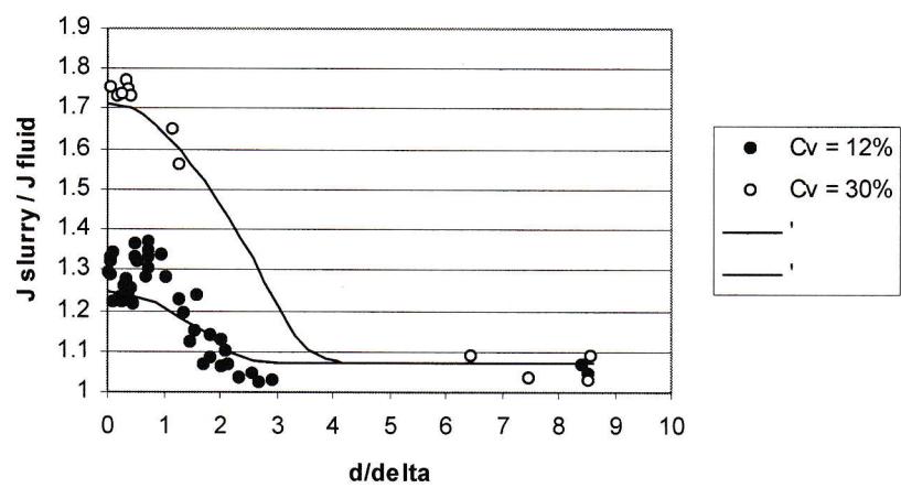
FIGURE 8 FINE AND COARSE COAL IN CLAY COAL CONCENTRATION 20% BY VOLUME 105 mm PIPE
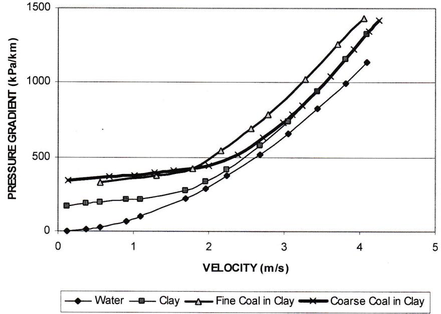
FIGURE 9 MINUS 300 MICRON BACKFILL TAILS
71% CONCENTRATION 146 mm PIPE