This HTML edition contains selectable text extracted from the original PDF. Layout-aware OCR was used to recover reading order, figures and equations; minor recognition errors may remain. Consult the PDF for the authoritative layout, figures and equations.
A New Analysis of the Turbulent Flow of Non-Newtonian Fluids
KENNETH C. WILSON
Department of Civil Engineering, Queen's University, Kingston, Ontario, Canada K7L 3N6
and
ALLAN D. THOMAS
Consulting Engineer, Newcastle N.S.W., Australia
A new analysis has been developed for the turbulent flow of non-Newtonian fluids. Based on enhanced viscosity effects at the small time and length scales of the dissipative micro-eddies, the analysis predicts a thickening of the viscous sub-layer tending to increase throughput velocity and thus promoting drag reduction. The required flow parameters can be determined directly from rheograms, without employing correlations based on pipe-flow data. The results give good descriptions of flows of fluids with both power-law and Bingham behaviour and explain a number of peculiarities of such flows.
On propose une nouvelle méthode d'analyse des écoulements de fluides non newtoniens. Cette analyse est fondée sur l'augmentation de la viscosité dans les microtourbillons (échelle de Kolmogorov) et permet de prédire un épaississement de la sous-couche viscosité. Il s'ensuit une augmentation de la vitesse d'écoulement et donc une réduction de la résistance due à la friction. Les paramètres nécessaires à cette analyse peuvent être directement obtenus à partir des rhéogrammes, l'utilisation de corrélations empiriques étant rendue inutile. Cette méthode a été testée avec des fluides de type plastique de Bingham et loi de puissance; elle permet de décrire avec réalisme le comportement des fluides ainsi que d'expliquer certaines de leurs particularités.
The flow of non-Newtonian fluids is reasonably well-understood only at low Reynolds numbers — for example, in the laminar range it is possible (at least for Bingham plastics and power-law fluids) to define an equivalent viscosity which produces the same relationship between friction factor and Reynolds number that is found for Newtonian flow. In the early stages of the study of turbulent flow of non-Newtonian fluids, it was hoped that an effective turbulent viscosity could likewise be defined in such a way as to give a unique relation between Reynolds number and friction factor for smooth-walled turbulent flow (D. G. Thomas, 1963b). Analysis of recent experimental evidence A. D. Thomas, 1983) shows that there is little likelihood that such a unique correlation can exist.
Before considering the velocity distribution for turbulent non-Newtonian flow it is appropriate to outline some of the features of non-Newtonian relationships for shear stress, , in terms of rate of strain, . Figure 1 shows the shape of a typical curve of this type and nomenclature has been made compatible with Dealey (1984). As distinct from the linear plot of a Newtonian fluid, for which , the non-Newtonian fluid does not have a constant viscosity. The viscosity, , is still defined as the ratio of to ; this represents the slope of a secant line joining the origin to any point of interest on the curve. Another quantity related to viscosity is the slope of a tangent to the curve of versus , denoted here as and referred to as "tangent viscosity" or "incremental viscosity".
Both two-parameter had three-parameter expressions for non-Newtonian behaviour can be found in the literature, with the two-parameter models having a considerable advantage in simplicity. An early and well-known instance is the Bingham-plastic model, equivalent to a linear approximation to the actual shape of the curve linking and .
The shear-stress intercept is called the yield stress, and the slope ("tangent" viscosity ) has a constant value. Hence, for any shear stress, , which is greater than , the velocity gradient can be obtained as
Since the left-hand side of this equation also equals , it follows that
As an alternate to the Bingham-plastic model, the straight-line fit can be applied to the logarithms of and , giving the power-law formulation
or
On differentiating to obtain the tangent viscosity it is found that, for all locations on the curve
In pipe flow (laminar or turbulent) the shear stress varies linearly from zero at the centre-line to a maximum, , at the pipe wall. Thus the velocity gradient, as given by Equations (1) or (4), is the greatest at the wall, where . For laminar flow of a Newtonian fluid, the variation of gradient across the section gives the well-known parabolic velocity profile, but for typical non-Newtonian behaviour ( or ) the laminar profile will be somewhat blunter, giving a smaller average velocity for the same conditions at the wall. As a result the "effective" viscosity , used to predict the discharge by means of the formula for laminar
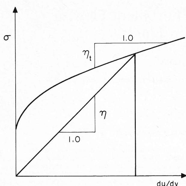
Figure 1 — Typical non-Newtonian rheogram.
Newtonian flow, must be somewhat larger than the viscosity which is applicable to conditions in the immediate vicinity of the wall (D. G. Thomas, 1963a).
For turbulent pipe flow, considerable idealization is employed, even for a Newtonian fluid (Reynolds, 1974). Thus the flow immediately adjacent to the pipe wall (assumed here to be hydraulically smooth) is analysed specifically as a viscous sub-layer. This thin sub-layer accounts for a large change in velocity because of its high strain rate, which is based on wall shear stress and viscosity and thus resembles the near-wall part of a laminar flow. Once the viscous sub-layer is passed, however, the turbulent velocity profile is much blunter than that of the laminar equivalent. The reduced velocity gradient is caused by turbulent momentum interchange, which is an inertial process, not a viscous one. Beyond the viscous sub-layer this produces an inertial layer typified by a logarithmic velocity profile.
If, for the same wall shear stress, the Newtonian fluid is replaced by a non-Newtonian one of the same density, major changes in velocity gradient would not be expected in the logarithmic zone. Also, the velocity gradient in the viscous sub-layer can be determined readily from the wall shear stress and the viscosity associated with this stress. If the thickness of the viscous sub-layer is assumed to be unchanged, then it would be expected that the friction factor for the non-Newtonian flow would be nearly the same as . This approach was followed by Eissenberg and Bogue (1964) and by Edwards and Smith (1980), and their work will be discussed later.
In fact, experimentally-determined friction factors often lie significantly below the Newtonian equivalents. This would now be expressed by the statement that typical non-Newtonian fluids have a significant drag-reduction effect. However, in the 1960's, when much of the early work on turbulent non-Newtonian flow was carried out, drag reduction studies were only beginning and there was no general awareness of this phenomenon. As a result, the rheologists of the day generally did not look to drag reduction, but simply sought some reduced effective viscosity which would give a larger Reynolds number and hence should
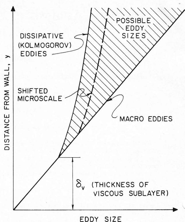
Figure 2 — Eddy scales in turbulent flow.
produce a smaller friction factor. Their choice generally fell on the "tangent" viscosity , which, as seen above, is smaller than . Nevertheless, no cogent reason has ever been adduced for the use of such a viscosity in the viscous sub-layer (or elsewhere in the flow). Recent work (A. D. Thomas, 1983) has shown that use of the tangent viscosity does not lead to correct prediction of the friction factor, but still gives overpredictions. It was also found that other attempts to deal with this discrepancy (to be discussed later in this paper) have not proved to be successful.
Drag reduction mechanisms
Better results may be sought by using what is now known of drag reduction mechanisms. In effect, two different types of drag reduction may occur, one affecting the logarithmic portion of the velocity profile and the other the thickness of the viscous sub-layer. The first type, often described as a changed von Karman coefficient, has been associated with the action of gravity on a cross-flow density gradient. In the atmosphere this typically arises from a temperature gradient (Webb, 1970), and in flumes it can be caused by varying concentration of suspended sand particles (Vanoni, 1946). The non-Newtonian fluids which are of interest here do not exhibit detectable density gradients, and thus will not be susceptible to this mechanism of drag reduction.
The remaining mechanism — thickening of the viscous sub-layer — is associated with the dramatic drag reduction obtained in aqueous flows by the addition of small quantities of certain long-chain molecules. It appears that these substances act by increasing the size of the smallest, dissipative, turbulent eddies. The phenomenon, as described by Lumley (1973, 1978), is illustrated on Figure 2, which graphs the distance from the wall, , in the vertical direction and representative eddy sizes in the horizontal direction. As shown, the size of the largest eddies (the macro scale of
turbulence) is directly proportional to the distance from the wall, while the size of the smallest eddies (the dissipative, or Kolmogorov, scale) is known to have a non-linear relation with distance from the wall, as indicated on the figure. At large values of the inertial macro-eddies are much larger than the dissipative micro-eddies, and between them is a whole range of turbulent eddy sizes, shown shaded on Figure 2. As the wall is approached, the range of possible eddy sizes shrinks until the size of the largest and smallest eddies are equal, which indicates the boundary of the turbulence. At this point equals , the thickness (in a statistical sense) of the viscous sub-layer.
The dashed line on Figure 2 shows that increasing the size of the dissipative micro-eddies leads to an increase in the viscous sub-layer thickness. If other quantities are unaffected this, in turn, will produce a higher mean velocity for the same wall shear stress, giving a lower friction factor. The explanation for the increase in the scale of dissipative eddies in non-Newtonian fluids lies in the nature of turbulent dissipation. It is generally accepted that new eddies tend to form at the macro scale, and at this size they experience very little viscous dissipation. Smaller eddies are produced from larger ones, mostly by stretching along the eddy axis (Tennekes and Lumley, 1972, Chapter 3). This "vortex stretching" process not only reduces eddy size but also increases angular velocities, and the combined effect results in smallest eddy sizes. Related to this is the concept of the "energy cascade" by which energy introduced at the largest eddy sizes moves from these through the inertial size ranges to the smallest eddies, where it is dissipated.
From this description it can be seen that energy dissipation in turbulent flow is not a true steady-state process. Unlike the steady conditions found in laminar flow, and approximated in the viscous sub-layer, turbulent flow involves a series of rapid dissipative events, as eddies drop from the inertial to the dissipative size range. There is an analogy between these two processes in fluid mechanics and steady-state versus dynamic loading in strength of materials. Just as the strain energy on applying a load is determined from the integral of the stress-strain curve (Timoshenko and MacCullough, 1949, Chapter 11), so the typical rate of energy dissipation of a turbulent eddy is represented by the integral of the curve of shear stress versus strain rate. Of course, for a Newtonian fluid this integral is merely the area of a triangle, given by or , but for a non-Newtonian fluid the area involved will generally be larger, as shown on Figure 1. The ratio of non-Newtonian to Newtonian areas (for the same values of and at the upper limit) is denoted by , and its evaluation in terms of the rheologic parameters will be dealt with later.
The increased area under the non-Newtonian curve does not imply a greater rate of energy dissipation, since the energy cascade dictates the energy dissipation rate which is imposed on the smallest eddies. Instead, the increased area indicates that, as far as dissipative eddies are concerned, the non-Newtonian fluid acts as if it were a Newtonian fluid with viscosity (which will give the same area under the curve, and hence the same dissipation rate as that for the non-Newtonian). Since the dissipation process imposes a constant-Reynolds-number relation on the smallest eddies, it follows that the product of eddy size and typical velocity for these eddies will be proportional to .
The scaling laws by which the length scale (and the velocity scale) of the micro-eddies vary within the inertial (loga-
rithmic) zone of the flow are known (Tennekes and Lumley, 1972, Chapter 5), but it is sufficient here to consider conditions at the interface between the inertial layer and the viscous sub-layer. At this point the length scales of the largest and smallest eddies effectively coincide, as shown on Figure 2, and the same applies to the typical velocities of these eddies, which must be proportional to the shear velocity , equal to . As this typical velocity can be considered as constant, and as it was seen that the product of velocity and eddy size varies with , then it follows that the minimum eddy size for a non-Newtonian fluid is larger than that for a Newtonian fluid (of the same ) by the factor . Based on the geometric relationship shown on Figure 2, it can be seen directly that the same factor applies to the thickness of the viscous sub-layer, .
Effect on velocity
Next, it is necessary to determine the effect of the thickened viscous sub-layer on the velocity profile. For this purpose the transition, or buffer layer, between the viscous sub-layer and the logarithmic zone need not be considered; instead the usual engineering approximation will be made, assuming that the linear profile of the viscous sub-layer meets the logarithmic profile where (Reynolds, 1974, Chapter 4). Within the viscous sub-layer conditions are taken as essentially steady-state, so that the viscosity , evaluated at is appropriate for a non-Newtonian fluid, and the velocity distribution, both Newtonian and non-Newtonian, is given by
The intercept with the logarithmic profile (at and ) is given, for the Newtonian case, by and . For the non-Newtonian case, with its thickened viscous sub-layer, 11.6 must be replaced by 11.6 .
In the logarithmic zone the general form of the velocity profile is given by
where 2.5 is the inverse of the von Karman coefficient. Substitution of and the value given above for yields the classic expression for the Newtonian case
For the non-Newtonian case this becomes
Since the area ratio (like the viscosity ) is evaluated for , the last two terms of Equation (9) will be constant throughout the pipe, and thus their contribution to the velocity ratio will apply equally to the ratio of the throughput velocity to . (Any constant velocity increase in the logarithmic zone will produce an equal increase in the core, or velocity-defect zone, and the viscous sub-layer comprises such a minute portion of the total area that variations here have no influence on the throughput velocity.)
The velocity represents the mean velocity for equivalent Newtonian flow, i.e. flow with the same for a Newtonian fluid with corresponding to the non-Newtonian value at . A final term, denoted here by , should be included to represent the effect on mean velocity
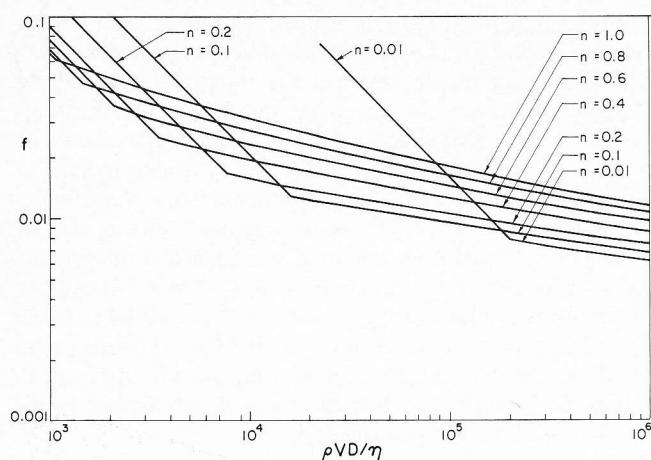
Figure 3 — Friction-factor prediction for power-law fluids.
ity, if any, of possible blunting of the velocity profile in the logarithmic or core regions of the flow. This gives the expression
As the flow in the logarithmic and core regions is governed by inertia, not viscosity, non-Newtonian viscosity per se should have virtually no effect here, implying a zero value for . However, non-Newtonians with a yield stress will have a velocity profile with a flattened core, and in this case will be greater than zero and should depend on (for convenience this ratio will be denoted by ). One reasonable way of approximating this effect is to assume that the logarithmic profile Equation (9) extends inwards only until the radius at which is reached. From there to the centreline, the velocity is assumed to remain constant. For such a profile it can be shown that
An alternate evaluation based on a parabolic velocity-defect law near the pipe centreline (Reynolds, 1974, p. 138) gave a different form for the expression for , but did not differ significantly in numerical value throughout the expected range of . It can be seen that for any fluid with , Equation (11) gives , as expected. (For a Newtonian fluid it is also the case that , so that all terms but the first drop from the right-hand side of Equation (10).)
Substitution of Equation (11) into Equation (10) gives a relationship of a general nature, which can readily be applied to those problems for which the wall shear stress is known in advance. The area ratio can, if necessary, be determined directly from the curve of shear stress versus shear rate; using the upper limit associated with the wall shear stress , which is appropriate since the typical eddy velocity is or . As the ratio equals , where is the Stanton-Moody friction factor, the process just described is equivalent to evaluating the friction factor.
For the particular case of the power law fluid discussed previously, it can be shown that equals , irrespective of the location of the upper limit for integration, and likewise . It follows that, for the power law fluid, Equation (10) can be rewritten as
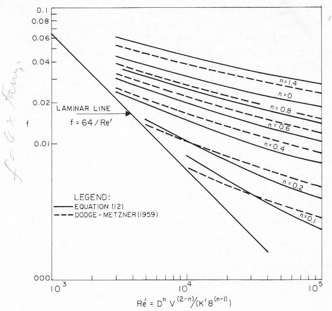
Figure 4 — Comparison with Dodge-Metzner (1959) correlation for power-law fluids.
Figure 3, which displays versus ( , where is evaluated at the wall shear stress), gives a more direct indication of the differences between Newtonian ( ) and non-Newtonian ( ) behaviour which are implied in Equation (12). In constructing this figure, has been evaluated using the smooth-wall expression which can be written
and the turbulent-flow lines have been terminated where they intercept the appropriate laminar-flow line. Figure 3 shows clearly that the predicted friction factor for turbulent flow of power-law fluids with will be less than that for a Newtonian fluid at the same Reynolds number .
As discussed in experiments on non-Newtonian flow are often correlated using the Bingham-plastic equation, it is also important to express Equation (10) in terms of the Bingham parameters. It can easily be shown that ( — equals , or ). When this, in combination with Equation (11), is substituted into Equation (10) a solution can be obtained without difficulty in cases where is known in advance. For other cases it is desirable to recast the equation in terms of two dimensionless parameters, the “plastic” shear Reynolds number , and the Hedstrom number . Using these parameters, the ratio is expressed as . The Newtonian velocity ratio of Equation (12) is then rewritten as
or, using Equation (2), and with
Combining Equations (10), (11) and (15) gives, for the Bingham-plastic formulation [for which ]
of as representing the "Newtonian" value of . When the sum of the remaining terms was plotted against , a maximum value of approximately 3.2 was found at of about 0.65. It follows that, for a particular value of , the largest is given by
This is so provided that is included in the portion of the constant-Hedstrom curve to the right of the laminar-turbulent intercept, which is the case for all (corresponding to and ). The right limb of the envelope on the diagram of friction factor versus plastic Reynolds number has been plotted on this basis on Figure 5. For smaller values of the envelope can be based on the intercept of the turbulent expression given above and the well known laminar expression
Points obtained at this intercept were used to plot the left limb of the envelope shown in Figure 5.
Comparison with experimental data and earlier theories
The theory just presented is applicable to all purely viscous fluids (Category I of Metzner, 1961), and it is not necessary to fit a rheological model since the area under the flow curve can, if necessary, be evaluated numerically. However the fitting of a model will often be convenient and the most common models — power-law and Bingham-plastic — will be used below in comparing the existing corpus of experimental results with the predictions of the new theory which has been developed above. Although three-parameter models such as the yield-power-law and the Powell-Eyring, together with more unusual two-parameter models such as the Casson, appear suitable for analysis by the new theory, discussion of these models will not be undertaken here. In addition, it should be noted that the theory cannot be applied immediately to suspensions containing coarse particles, for which additional effects must be taken into account (A. D. Thomas, 1983).
POWER-LAW MODEL
For power law fluids the classic work of Dodge and Metzner (1959) provides a valuable datum for comparison. Figure 4 shows a plot of friction factor versus the Metzner-Reed (1955) Reynolds number , given by
where .
The full lines on Figure 4 indicate the predictions using the new theory and the dashed lines are plots of Dodge and Metzner's empirical correlation formulas. Significant agreement between the Newtonian line ( ) but showing increasing deviation below that line with decreasing .
The predictions of the new analysis fall 5 to 15 percent below the Dodge and Metzner (1959) correlations, and are rather similar to the formulations of Clapp (1961) and Torrance (1963), both of which fall some 15% below Dodge and Metzners' for and some 20% below for , based on a range of Reynolds number from to .
The alternate presentation of new analysis shown on Figure 3 uses the secant viscosity based on the prevailing wall shear stress. It was noted previously that Eissenberg and
Bogue (1964) and Edwards and Smith (1980) also used the secant viscosity. For mildly non-Newtonian fluids ( ) they found that this approach generally resulted in velocity profiles and friction factors identical to the Newtonian values, whereas for more highly non-Newtonian fluids ( ) this agreement was generally not found. These authors postulated the existence of some wall-slip or drag-reduction effect, but did not attempt to analyze the mechanism involved. It will now be shown how most of these apparent anomalies can be explained by the new analysis.
On considering Figure 3 it is seen that for the predicted friction factors fall below the Newtonian value, but the divergence is no more than 6 or 7 percent. Experimental uncertainty would often be of this order, and it is understandable that the Newtonian value could be assumed to appear (1964) for their high concentration thoria suspensions can be dealt with next. For these slurries the measured turbulent velocity profiles indicate consistently exceeding the Newtonian value by about 2.4 (see their Figure 6). The laminar flow curves for these slurries can be approximated by a power law with , for which Equations (10) and (11) predict a constant increase in turbulent by 1.91. In view of the considerable scatter of the data this can be considered as essential agreement with the measured increase. Similarly, the observed friction factors which were some 15% less than the Newtonian line are in good agreement with the 18% reduction predicted by the new analysis (see Figure 3).
The apparently anomalous data of other authors cited by Edwards and Smith (1980) are likewise explained. Thus the data from Shaver (1957), with fall some 15 percent below the Newtonian friction factor line, which is in excellent agreement with present predictions. Similarly Dodge's (1961) data for 0.2% and 0.3% carbopol ( ) and ) which fall respectively some 5% and 18% below the Newtonian line are in reasonable agreement with present predictions (16% and 23%).
In summary, it can be concluded that the new analysis provides an adequate prediction of the behaviour of power-law fluids.
BINGHAM-PLASTIC MODEL
For the Bingham model the predictions have been given in Figure 5 as friction factor versus Reynolds number based on the plastic viscosity, and with the Hedstrom number, , as parameter. The first thing to note is that the theory predicts a maximum deviation below the Newtonian line of between 15 and 25%, occurring at or shortly after laminar-turbulent transition. Thereafter the predicted curve approaches the Newtonian line, effectively reaching it at a Reynolds number some five times the transition value. This rather rapid convergence to the Newtonian line is in very close agreement with the prediction of Tomita (1959, 1961), and the data given by Bain and Bonnington (1970), for chalk slurries show similar behaviour (see Figure 5).
The same trend has also been found in a sizeable body of suspension data which has been analysed, not as a Bingham plastic, but as a power-law fluid. For example, Metzner and Reed (1955) show data for a variety of suspensions for which the friction factor virtually joins the Newtonian line at a generalized Reynolds number about 3.5 to 5.5 times the laminar-turbulent transition value. Similarly, Kemblowski
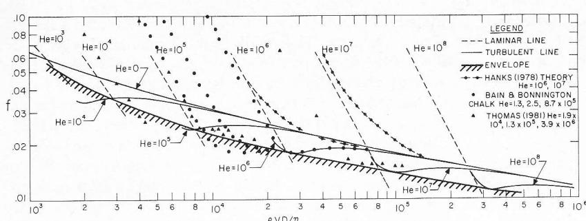
Figure 5 — Comparison with Bingham-plastic data and theory of Hanks (1978).
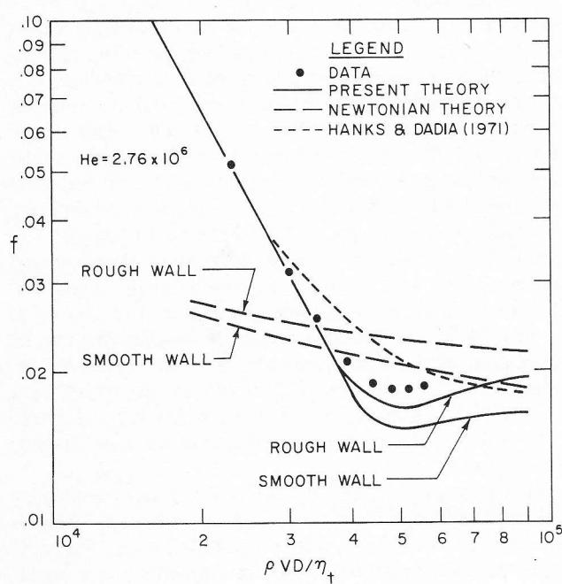
Figure 6 — Comparison with data for limestone in 206 mm pipe.
and Kolodziejski (1973) presented data for a 30% kaolin suspension velocity and that required to reach the Newtonian line. All these sets of data are in good accord with the predictions of the new analysis.
The theory of Hanks and Dadia (1971) predicts a different pattern with the Bingham line nearly paralleling the Newtonian line, and other experimental data, e.g. Caldwell and Babbitt (1941), Wilhelm et al. (1939), D. G. Thomas (1960, 1962) and A. D. Thomas (1981) show the same trend. (The data of the latter for a kaolin clay slurry in 7.2, 19 and 105 mm pipes is shown in Figure 5.) The existence of two populations differing in behaviour implies that more detailed analysis is needed, possibly requiring a three-parameter rheologic model. This problem will be addressed in the near future.
Another feature of the present theory is, as previously discussed, the different behaviour predicted for Hedstrom numbers above and below . Below this value of the predicted friction factor for turbulent flow shows a monotonous approach towards the Newtonian line with increasing Reynolds number. For the predicted initial trend following the transition to turbulence is to drop away from the Newtonian line until a maximum deviation is reached (at ) whence the trend alters, move back up toward the Newtonian line. This behaviour
bears a slight similarity to the "extended transition" region predicted by Hanks and Dadia (1971) for Hedstrom numbers in excess of about . However the behaviour which they predict is significantly different, showing the beginning of deviation from the laminar line, at friction factors well above the Newtonian turbulent line, as shown on Figure 6. It should be noted that the data plotted on Figure 6 do not show this type of transition region. Mishra and Tripathi (1971) had already remarked on the discrepancy between Hanks' theory and published data. It is also significant that Bowen (1961), who considered both power law and Bingham plastics, concluded that no significant transition zone existed for Bingham plastics.
The predicted change in behaviour at is partly substantiated by the data of D. G. Thomas (1960, 1962) who correlated data from a number of different slurries tested in pipes from 3 to 26 mm in diameter. He found differing behaviour for yield stress values above and below 25 Pa. For slurries having yield stress below 25 Pa the friction factor—Reynolds number plot converged towards the Newtonian line whilst for high-yield-stress slurries it diverged. Using typical values of density and plastic viscosity for his 25 Pa slurry, the relevant Hedstrom numbers for the pipe sizes of these experiments are found to range from to . These limits encompass the value of at which the new analysis predicts a behaviour change, and thus it appears that the present analysis can explain the change in behaviour observed by D. G. Thomas (1960, 1962).
Another feature of Hanks and Dadia's (1971) theory which is not in agreement with the new theory is the predicted effect of Hedstrom number on the shape of the curve of friction factor versus plastic Reynolds number. As noted previously, their theory predicts a turbulent friction factor relation which becomes parallel to the Newtonian line at Reynolds numbers larger than the transition range. For a Hedstrom number of their prediction (for large Reynolds number) lies some 40% below the Newtonian line, but the predicted difference decreases with increasing Hedstrom number, and for their prediction coincides with the Newtonian line. The original prediction indicated a further rise of above the Newtonian line at higher Hedstrom numbers, but more recently Hanks (1978) reappraised the data used and modified the theory to give friction factors below the Newtonian line for all values of . The new analysis that has been presented above does not predict any equivalent rise with increasing , and although A. D. Thomas (1983) has shown that available data indicate a slight effect when the change in is due to a change in pipe diameter, as seen for the kaolin data on Figure 5, the data do not correspond to Hanks' (1978) prediction. It was noted by Lumley (1973, p. 270) that a similar diameter effect is
found in dilute polymer flow, where it may be associated with a time scale ratio.
Although all turbulent flow, this is not required by the present analysis since the effect of wall roughness (in the transition zone between the smooth and fully rough cases) can be incorporated in the first term of Equation (10). It is of interest to note the effect of wall roughness on some results for a minus 300 micron limestone slurry. 1 These data, for a 206 mm pipe, are shown in Figure 6. This particular slurry fitted the Bingham model with a yield stress of 7.92 Pa and a plastic viscosity of 14.1 mPas. The prediction of the present theory with a smooth-pipe assumption is seen to lie well below the data. However tests with water revealed a relative roughness for this pipe of 0.00079 which, in this Reynolds number range, puts the water friction factor some 12% above the smooth, pipe value. Increasing the smooth pipe value by the appropriate ratio results in the predicted "rough wall" curve shown. Agreement is now within about 8%, and the data are seen to follow a trend very similar to that of the predicted curve. For comparison, the Hanks' (1978) prediction for this Hedstrom number ( ) is shown with the pronounced "extended transition" data do not follow Hanks' prediction.
Although there is lack of complete agreement both between different theories and between different sets of data which have been fitted to the Bingham model, the new analysis appears to explain a number of experimentally observed phenomena which occur with Bingham fluids. The remaining problem — why some data are seen to converge rather rapidly towards the Newtonian line as predicted by the theory whilst other data tend to lie parallel — may require consideration of time-dependent effects or the use of three-parameter rheologic models. This matter will be addressed in the near future.
Conclusions
A new analysis has been developed for the turbulent pipe flow of any viscous non-Newtonian fluid. It is based on velocity profile alteration (drag reduction) associated with thickening of the viscous sub layer, and the flow parameters are determined directly from rheograms, without pipe-flow data. It has been shown to give a good description of flows of fluids with both power-law and Bingham behaviour and to explain a number of peculiarities of such flows. The authors recommend its use for non-Newtonian fluids and colloidal suspensions.
Nomenclature
| = internal diameter of pipe, m | |
| = Stanton-Moody friction factor | |
| = Hedstrom number ( ) | |
| = coefficient in power-law model (see Equation (3)) | |
| = coefficient in Equation (19) ( ) | |
| = exponent in power-law model | |
| = Reynolds number ( ) | |
| = Metzner-Reed Reynolds number (see Equation (13)) | |
| = "plastic" shear Reynolds number ( ) |
| = velocity, m/s | |
| = time-averaged velocity at a point, m/s | |
| = velocity at edge of viscous sub-layer (time averaged), m/s | |
| = shear velocity ( ) | |
| = throughput velocity (discharge/pipe area), m/s | |
| = throughput velocity for equivalent Newtonian flow, m/s | |
| = distance from boundary, m |
Greek letters
| = ratio of rheogram areas: non-Newtonian/Newtonian | |
| = thickness of viscous sub-layer, m | |
| = viscosity ( ), Pa·s | |
| = "effective" viscosity based on equivalent laminar Newtonian flow, Pa·s | |
| = "tangent" or "incremental" viscosity, Pa·s | |
| = stress ratio ( ) | |
| = fluid density, kg/m 3 | |
| = shear stress, Pa | |
| = yield stress, Pa | |
| = term in dimensionless throughput velocity equation (see Equations (10), (11)) |
References
Bain, A. G. and S. T. Bonnington, "The Hydraulic Transport of Solids by Pipeline", Pergamon Press, Oxford (1970).
Bowlen, R. L., "Scale-up for Non-Newtonian Fluid Flow: Part 4, Designing Turbulent-Flow Systems", Chem. Eng. 68(15), July 24, 143–150 (1961).
Caldwell, D. H. and H. E. Babbitt, "Flow of Muds, Sludges and Suspensions in Circular Pipe", Ind. Eng. Chem. 33, 249 (1941).
Clapp, R. M., "Turbulent Heat Transfer in Pseudo-Plastic Non-Newtonian Fluids", Int. Developments in Heat Transfer, A.S.M.E., Part III, Sec. A, 652 (1961).
Dealy, J., "Official Nomenclature for Material Functions Describing the Response of a Viscoelastic Fluid to Various Shearing and Extensional Deformations", J. Rheol. 28, 181 (1984).
Dodge, D. W., Ph.D. Thesis, Univ. of Delaware, Newark, Delaware (1961).
Dodge, D. W. and A. B. Metzner, "Turbulent Flow of Non-Newtonian Systems", AIChE J. 5, 189 (1959).
Edwards, M. F. and R. Smith, "The Turbulent Flow of Non-Newtonian Fluids in the Absence of Anomalous Wall Effects", J. Non-Newtonian Fluid Mech. 7, 77 (1980).
Essenberg, D. M. and D. C. Bogue, "Velocity Profiles of Thoria Suspensions in Turbulent Pipe Flow", AIChE J. 10, 723 (1964).
Hanks, R. W., "Low Reynolds Number Turbulent Pipeline Flow of Pseudo Homogeneous Slurries", Proc. Hydrotransport 5 Conf., Hanover, GFR C2-23 (1978).
Hanks, R. W. and B. H. Dadia, "Theoretical Analysis of the Turbulent Flow of Non-Newtonian Slurries in Pipes", AIChE J. 17, 554 (1971).
Kemblowski, A. and J. Kolodziejski, "Flow Resistances of Non-Newtonian Fluids in Transitional and Turbulent Flow", Int. Chem. Eng. 13, 265 (1973).
Lumley, J. L., "Poly Reaction in Turbulent Flow by Polymer Additives", Poly Sci., Macromol. Rev. 7, A. Peterlin (Ed.), Interscience, New York, pp. 263–290 (1973).
Lumley, J. L., "Two-Phase and Non-Newtonian Flow", in "Turbulence", P. Bradshaw (Ed.), Topics in Applied Physics, Vol. 12, Springer-Verlag, Berlin (1978), Chap. 7.
Metzner, A. B., "Flow of Non-Newtonian Fluids", Section 7, "Handbook of Fluid Mechanics", Ed. V. Streeter, McGraw-Hill, New York (1961).
Metzner, A. B. and J. C. Reed, "Flow of Non-Newtonian Fluids — Correlation of the Laminar, Transition and Turbulent Flow Regimes", AIChE J. 1, 434 (1955).
1 Proprietary data of Slurry Systems Pty. Ltd., North Sydney, Australia.
Mishra, P. and G. Tripathi, "Transition from Laminar to Turbulent Flow of Purely Viscous Non-Newtonian Fluids in Tubes", Chem. Eng. Sci. 26 , 915 (1971).
Reynolds, A. J., "Turbulent Flows in Engineering", John Wiley & Sons, New York (1974).
Shaver, R. G., D.Sc. Thesis, M.I.T., Cambridge, Mass. (1957).
Tennekes, H. and J. L. Lumley, "A First Course in Turbulence", MIT Press, Cambridge, Mass. (1972).
Thomas, A. D., "Slurry Pipeline Rheology", 2nd National Conf. on Rheology, Sydney, Aust. (1981).
Thomas, A. D., "Turbulent Pipe Flow of Bingham Plastics", 3rd National Conf. on Rheology, Melbourne, Aust. (1983).
Thomas, D. G., "Heat and Momentum Transport Characteristics of Non-Newtonian Aqueous Thorium Oxide Suspensions", AIChE J. 6 , 631 (1960).
Thomas, D. G., "Transport Characteristics of Suspensions: Part IV Friction Loss of Concentrated Flocculated Suspensions in Turbulent Flow", AIChE J. 8 , 266 (1962).
Thomas, D. G., "Non-Newtonian Suspensions: Part I, Physical Properties and Laminar Transport Characteristics", Ind. and Eng. Chem. 55 , 18 (1963a).
Thomas, D. G., "Non-Newtonian Suspensions: Part II, Turbulent Transport Characteristics", Ind. Eng. Chem. 55 , 27 (1963b).
Timoshenko, S. and G. H. MacCullough, "Elements of Strength of Materials", 3rd Ed. Van Nostrand, Princeton, N.J. (1949).
Tomita, Y., "A Study of Non-Newtonian Flow in Pipelines", Bulletin J.S.M.E. 2 , 469 (1959); 4 , 77 (1961).
Torrance, B. McK., "Friction Factors for Turbulent Non-Newtonian Fluid Flow in Circular Pipes", S. Afr. Mech. Eng. 13 , 89 (1963).
Vanoni, V. A., "Transportation of Suspended Sediment by Water", Trans. Am. Soc. Civ. Eng. 5 , 111 (1946).
Webb, E. K., "Profile Relationships, the Log-Linear Range and Extension to Strong Stability", Q.J.R. Meteorol. Soc. 96 , 67-90 (1970).
Wilhelm, R. H., D. M. Wroughton and W. F. Loeffel, "Flow of Suspensions through Pipes", Ind. Eng. Chem. 31 , 622 (1939).
Manuscript received June 28, 1984; revised manuscript received January 28, 1985; accepted for publication March 1, 1985.